6 Chlorophyll-a

Published

2025-04-15T03:25

What is it?

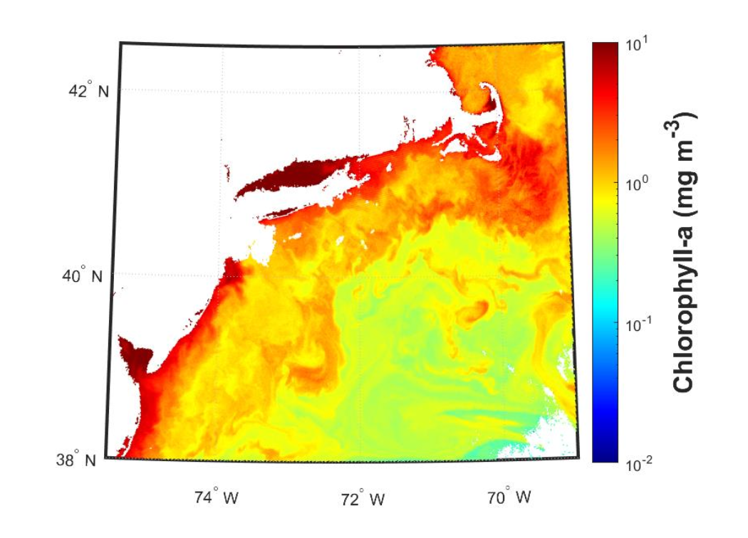
Chlorophyll-a (Figure 6.1) is a pigment contained within all phytoplankton and cyanobacteria cells. It is an estimate of algal biomass that is used for mapping the distribution of phytoplankton over time and space.

How does it impact Aquaculture/Fisheries?

Chlorophyll-a is a useful proxy of the biomass of phytoplankton in the water, the food source to filter feeding organisms and zooplankton. This parameter has been utilized for aquaculture siting, farm aquaculture resource management models, HAB forecasts, species distribution models (fish, mammals, top predators, other highly migratory species), ecosystem models, ecosystem status monitoring, as a predictor of unregulated fishing activity, and more.

What are the limitations/caveats?

Currently, chlorophyll-a can be confused with other dissolved materials in the water, and it can be over-estimated in coastal regions, particularly in areas with river inputs or sediment resuspension. It is useful to note that the amount of chlorophyll-a in a phytoplankton cell can vary substantially based on physiological and environmental conditions, and thus, it is possible that increases in chlorophyll-a do not explicitly represent increases in biomass.

Does HYPERSPECTRAL directly improve/enable this product?

Having more information about the other components of the water will help separate the living from non-living components, and should improve the performance of the chlorophyll- a product substantially. Many efforts at improving chlorophyll-a have been attempted using regional tuning methods, generalized additive models, and dynamic optical water types, or applying machine learning techniques and neural networks, but lack unified community consensus or adoption.

Figure 6.1: Projection of PACE-derived chlor_a in the North Atlantic Ocean; May 13, 2024.

Python

Code to access data

%%time
# 1 minute or so
# Authenticate to NASA
%%time
# Authenticate to NASA
import earthaccess
auth = earthaccess.login(strategy="interactive", persist=True)
    
# (xmin=-73.5, ymin=33.5, xmax=-43.5, ymax=43.5)
bbox = (-75.5, 38.0, -69.0, 42.5)
import earthaccess
results = earthaccess.search_data(
    short_name = "PACE_OCI_L2_BGC",
    temporal = ("2024-05-13", "2024-05-13"),
    bounding_box = bbox
)
fileset = earthaccess.open(results);

# load data
import xarray as xr
ds = xr.open_dataset(fileset[0], group="geophysical_data")

# Add coords
# Add coords
nav = xr.open_dataset(fileset[0], group="navigation_data")
nav = nav.set_coords(("longitude", "latitude"))
dataset = xr.merge((ds["chlor_a"], nav.coords))

# Subset
chla_box = dataset.where(
    (
        (dataset["latitude"] > 38.0)
        & (dataset["latitude"] < 42.5)
        & (dataset["longitude"] > -75.5)
        & (dataset["longitude"] < -69.0)
    ),
    drop = True
)

Make one plot

import matplotlib.pyplot as plt
from matplotlib.colors import LogNorm

chl = chla_box["chlor_a"].where(chla_box["chlor_a"] > 0)

plot = plt.pcolormesh(
    chla_box["longitude"], chla_box["latitude"], chl,
    cmap="jet", norm=LogNorm(vmin=1e-2, vmax=1e1), shading="auto"
)
cbar = plt.colorbar(plot)
cbar.set_label("Chlorophyll-a (mg m⁻³)", fontsize=16, fontweight="bold")

plt.xlim(-75.5, -69.0)
plt.ylim(38.0, 42.5)
plt.xlabel("Longitude")
plt.ylabel("Latitude")
plt.title("Chlorophyll-a (Log Scale)")

plt.show()