7  Phytoplankton carbon

What is it?

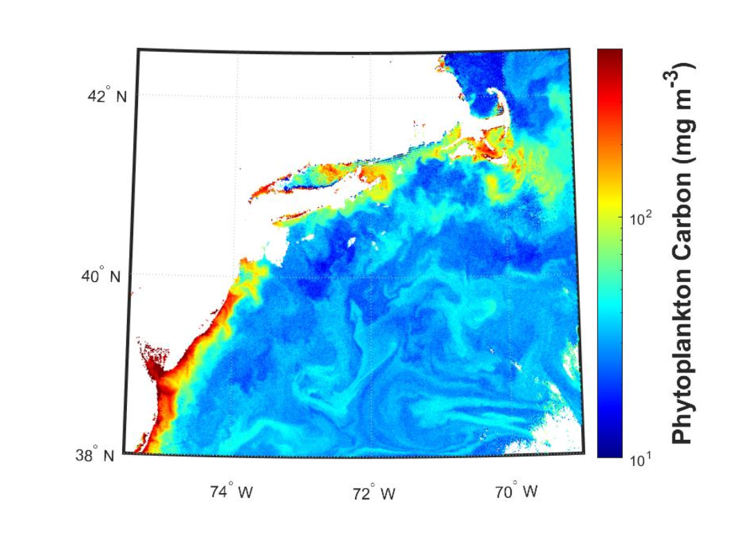
The phytoplankton carbon product (Figure 7.1) expresses the concentration of phytoplankton in terms of carbon concentration, instead of chlorophyll-a. Contrasting from the chlorophyll- a product, phytoplankton carbon is derived from an empirical relationship to the particle backscattering properties (see Product 7) of the water.

How does it impact Aquaculture/Fisheries?

Some fisheries applications may prefer to work in units of carbon biomass instead of pigment-based (i.e., chlorophyll-a) biomass. A constant chlorophyll-a value can represent a wide array of cell concentrations, due to environmental conditions and individual cell physiology/stress. For example, individual phytoplankton can produce more chlorophyll- a/cell in low-light conditions without changing the actual number of cells. The carbon product is not subject to these variations, and is a more direct indicator of phytoplankton biomass. Modelers may also be interested in computing a carbon to chlorophyll ratio to tease out environmental or species variations, and this is obtained as carbon_phyto ÷ chlor_a.

What are the limitations/caveats?

This product was empirically tuned with field data, but it is not currently representative of optically complex waters. The performance in coastal regions remains untested. This product relies on the “inherent optical property (IOP)” suite of ocean color products, and thus can sometimes fail to arrive at a solution (i.e., no data) in waters with extreme scattering or chromophoric dissolved organic matter (CDOM) concentrations.

Does HYPERSPECTRAL directly improve/enable this product?

Operational improvements to IOP backscatter products using hyperspectral data are anticipated, but still in development (at the time of this publication).

Figure 7.1: Projection of PACE-derived carbon_phyto in the North Atlantic Ocean; May 13, 2024.

Python

Code to access data

%%time
# 1 minute or so
# Authenticate to NASA
%%time
# Authenticate to NASA
import earthaccess
auth = earthaccess.login(strategy="interactive", persist=True)
    
# (xmin=-73.5, ymin=33.5, xmax=-43.5, ymax=43.5)
bbox = (-75.5, 38.0, -69.0, 42.5)
import earthaccess
results = earthaccess.search_data(
    short_name = "PACE_OCI_L2_BGC",
    temporal = ("2024-05-13", "2024-05-13"),
    bounding_box = bbox
)
fileset = earthaccess.open(results);

# load data
import xarray as xr
ds = xr.open_dataset(fileset[0], group="geophysical_data")

# Add coords
# Add coords
nav = xr.open_dataset(fileset[0], group="navigation_data")
nav = nav.set_coords(("longitude", "latitude"))
dataset = xr.merge((ds["carbon_phyto"], nav.coords))

# Subset
carbon_phyto_box = dataset.where(
    (
        (dataset["latitude"] > 38.0)
        & (dataset["latitude"] < 42.5)
        & (dataset["longitude"] > -75.5)
        & (dataset["longitude"] < -69.0)
    ),
    drop = True
)

Make one plot

import matplotlib.pyplot as plt
from matplotlib.colors import LogNorm

cp = carbon_phyto_box["carbon_phyto"].where(carbon_phyto_box["carbon_phyto"] > 0)

plot = plt.pcolormesh(
    carbon_phyto_box["longitude"], carbon_phyto_box["latitude"], cp,
    cmap="jet", norm=LogNorm(vmin=1e1, vmax=500), shading="auto"
)
cbar = plt.colorbar(plot)
cbar.set_label("Phytoplankton Carbon (mg m⁻³)", fontsize=16, fontweight="bold")

plt.xlim(-75.5, -69.0)
plt.ylim(38.0, 42.5)
plt.xlabel("Longitude")
plt.ylabel("Latitude")
plt.title("Phytoplankton Carbon (Log Scale)")

plt.show()