13  Remote sensing reflectance (Rrs)

What is it?

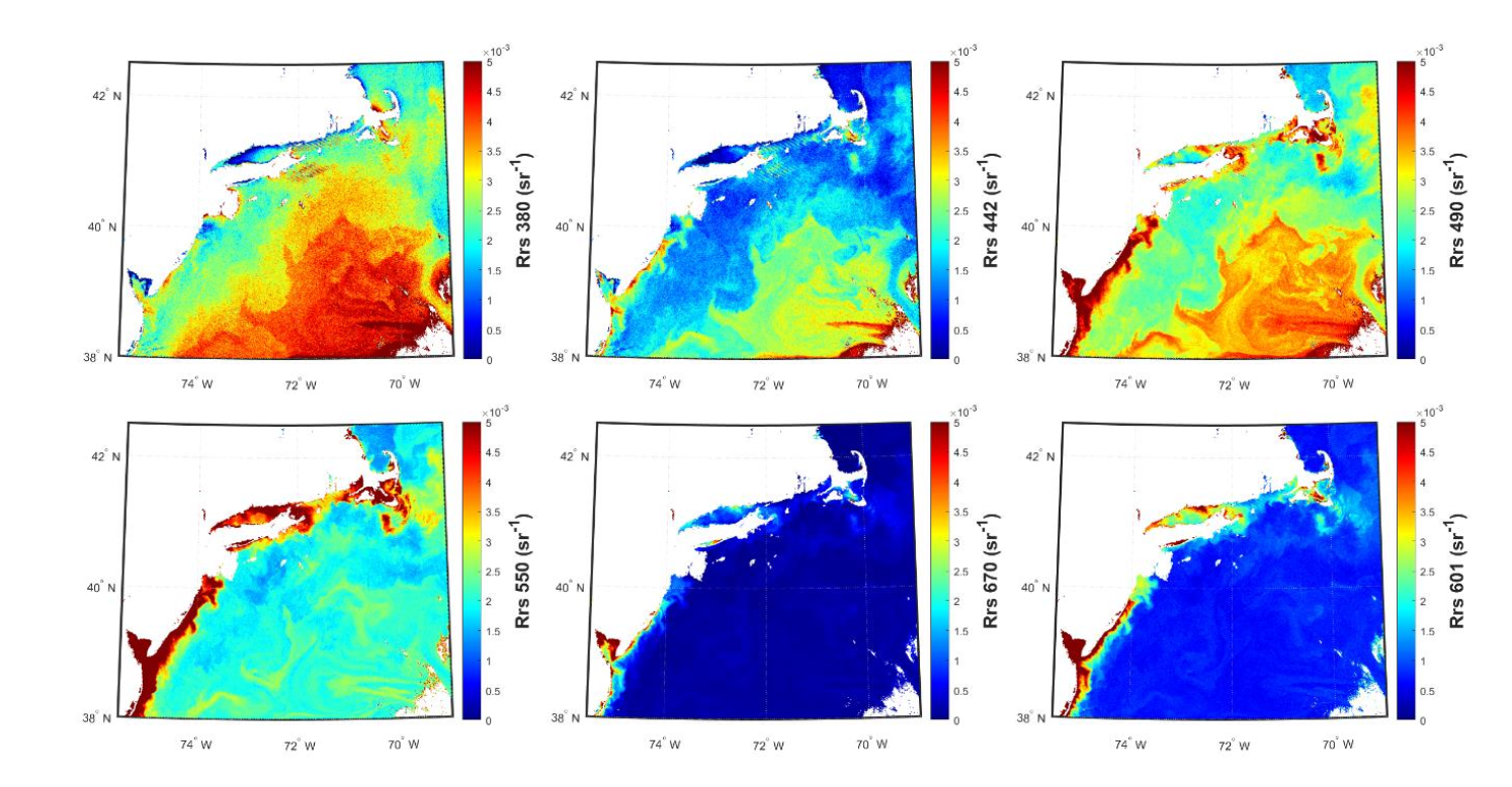
The remote sensing reflectance is the base unit by which most ocean color algorithms are built on. It is a direct measure of the water-leaving reflectance, after the atmosphere and surface reflectance effects have been removed. Each wavelength of color has its own reflectance value.

How does it impact Aquaculture/Fisheries?

These products may be preferred for advanced users who want to customize or build their own products for a regional/local application. This raw color information removes any the elements of uncertainty introduced by assumptions made during “product” development. If there are subtle features in the color reflectance spectrum that are unique to a phytoplankton species, this is currently the only set of products that will retain this information, though it is (currently) up to the user to determine what those features are. Some published algorithms for Harmful Algal Blooms can be reconstructed using the reflectance channels (see section 3).

What are the limitations/caveats?

The remote sensing reflectance is subject to uncertainties introduced in the removal of the atmospheric signal. These products may underperform, or be expressed as negative values, especially in areas with complex aerosol loadings (near urban areas), or in near-coastal regions.

Does HYPERSPECTRAL directly improve/enable this product?

For context, relative to MODIS (10 color bands) or VIIRS (5 color bands), PACE offers 120 visible color bands (+ additional UV bands) by which to develop algorithms from. PACE Science and Applications Team members are working to improve the removal of the atmosphere, and thus improve the reflectance product.

Python

Code to access data

%%time
# 1 minute or so
# Authenticate to NASA
import earthaccess
auth = earthaccess.login(strategy="interactive", persist=True)
    
# (xmin=-73.5, ymin=33.5, xmax=-43.5, ymax=43.5)
bbox = (-75.5, 38.0, -69.0, 42.5)
import earthaccess
results = earthaccess.search_data(
    short_name = "PACE_OCI_L2_AOP",
    temporal = ("2024-05-13", "2024-05-13"),
    bounding_box = bbox
)
fileset = earthaccess.open(results);

# load data
import xarray as xr
ds = xr.open_dataset(fileset[0], group="geophysical_data")

# Add coords
nav = xr.open_dataset(fileset[0], group="navigation_data")
nav = nav.set_coords(("longitude", "latitude"))
wave = xr.open_dataset(fileset[0], group="sensor_band_parameters")
wave = wave.set_coords(("wavelength_3d"))
dataset = xr.merge((ds["Rrs"], nav.coords, wave.coords))

# Subset
rrs_box = dataset.where(
    (
        (dataset["latitude"] > 38.0)
        & (dataset["latitude"] < 42.5)
        & (dataset["longitude"] > -75.5)
        & (dataset["longitude"] < -69.0)
    ),
    drop = True
)

Make one plot

import matplotlib.pyplot as plt

rrs = rrs_box["Rrs"].sel(wavelength_3d = 380)
plot = rrs.plot(x="longitude", y="latitude", cmap="jet", vmin=0, vmax=0.005)

# Set x and y limits
plot.axes.set_xlim(-75.5, -69.0)
plot.axes.set_ylim(38.0, 42.5)

# Customize colorbar label
wave_string = "380"  # or str(wavelength) if dynamic
plot.colorbar.set_label(f"Rrs {wave_string} (sr⁻¹)", fontsize=16, fontweight="bold")

plt.show()

Code to generate 6 panel figure

import matplotlib.pyplot as plt
import matplotlib.colors as colors

# List of wavelengths to plot
wavelengths = [380, 442, 490, 550, 670, 588]

# Create figure and axes
fig, axes = plt.subplots(3, 2, figsize=(12, 12), constrained_layout=True)
axes = axes.flatten()

# Loop through wavelengths and plot
for i, wl in enumerate(wavelengths):
    ax = axes[i]
    
    # Extract Rrs and mask zeros (for log or safety)
    rrs = rrs_box["Rrs"].sel(wavelength_3d=wl)
    
    # Plot onto the provided axis
    img = rrs.plot(
        ax=ax,
        x="longitude",
        y="latitude",
        cmap="jet",
        vmin=0,
        vmax=0.005,
        add_colorbar=False  # We'll add our own
    )
    
    # Set limits
    ax.set_xlim(-75.5, -69.0)
    ax.set_ylim(38.0, 42.5)
    
    # Add colorbar
    cbar = fig.colorbar(img, ax=ax, orientation="vertical", shrink=0.8)
    cbar.set_label(f"Rrs {wl} (sr⁻¹)", fontsize=12, fontweight="bold")
    
    # Optional: title or annotation
    ax.set_title(f"Wavelength {wl} nm")

# Turn off unused axes (if any)
for j in range(len(wavelengths), len(axes)):
    fig.delaxes(axes[j])

plt.show()