3 - Stamen Map • basics

This example assumes that you have a sample raster. You can load the sample one or go to the download data vignette to download your own. sample_raster is a demo SST raster and data frame.

Load the sample data.

data("sample_raster", package="basics")
df <- sample_raster$df
ras <- sample_raster$raster
lons <- sample_raster$lons
lats <- sample_raster$lats

Load the needed packages for plotting.

require(raster)

## Loading required package: raster

## Loading required package: sp

require(ggplot2)

## Loading required package: ggplot2

Stamen map the gridded data

# Give coordinates for map
bbox <- c(left = lons[1], bottom = lats[1], right = lons[2], top = lats[2])
# Get stamen map
ocean_map <- ggmap::get_stamenmap(bbox, zoom = 5, maptype = "terrain")

## Source : http://tile.stamen.com/terrain/5/3/10.png

## Source : http://tile.stamen.com/terrain/5/4/10.png

## Source : http://tile.stamen.com/terrain/5/5/10.png

## Source : http://tile.stamen.com/terrain/5/3/11.png

## Source : http://tile.stamen.com/terrain/5/4/11.png

## Source : http://tile.stamen.com/terrain/5/5/11.png

## Source : http://tile.stamen.com/terrain/5/3/12.png

## Source : http://tile.stamen.com/terrain/5/4/12.png

## Source : http://tile.stamen.com/terrain/5/5/12.png

If you wanted to change the color of the ocean, you could do this.

attr_om <- attr(ocean_map, "bb")    # save attributes from original

# change ocean color in raster
ocean_map[ocean_map == "#99B3CC"] <- "#F5F5F5"
class(ocean_map) <- c("ggmap", "raster")
attr(ocean_map, "bb") <- attr_om

require(ggmap)

## Loading required package: ggmap

## Google's Terms of Service: https://cloud.google.com/maps-platform/terms/.

## Please cite ggmap if you use it! See citation("ggmap") for details.

# Plot
gg <- ggmap(ocean_map) +
  geom_tile(aes(lon, lat, fill = sst),
            data = df, na.rm = TRUE) +
  scale_fill_gradient2(midpoint = mean(df$sst, na.rm = TRUE),
                       low = "blue",
                       mid = "white",
                       high = "red",
                       na.value = "transparent") +
  labs(x = NULL,
       y = NULL,
       fill = "Celcius",
       title = "Sea Surface Temperature (SST)")
gg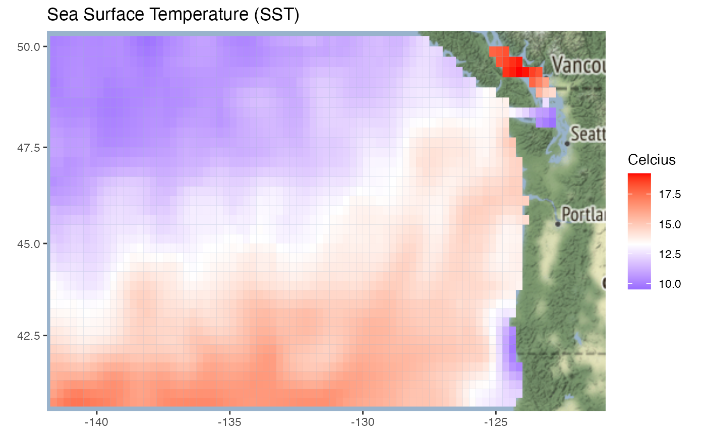

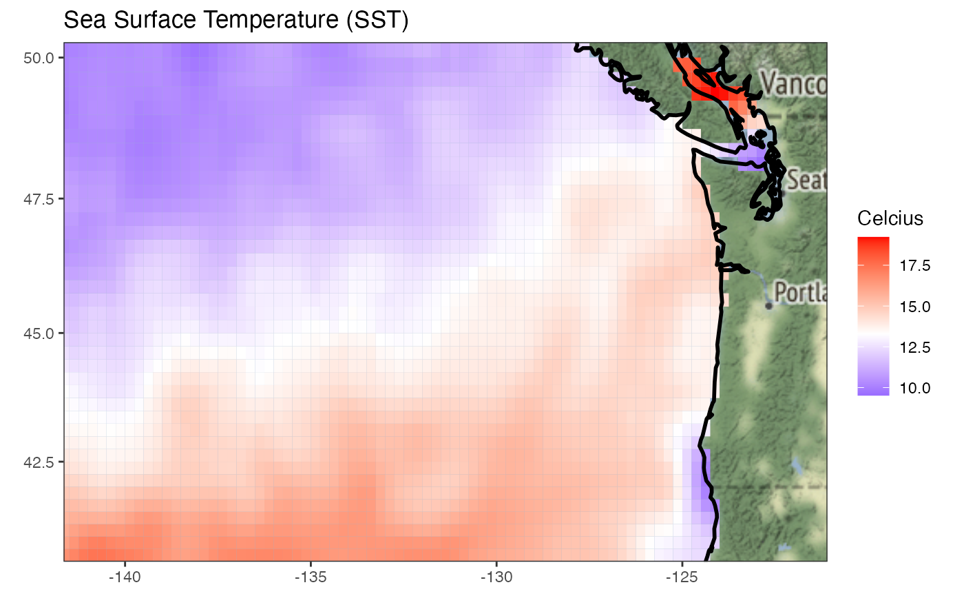
Adding a coastline

Download a coast

coast <- rnaturalearth::ne_coastline(scale = 50, returnclass = "sp")
wa_or_coast <- raster::crop(coast, raster::extent(lons[1], lons[2], lats[1], lats[2]))
plot(wa_or_coast)

## Warning in wkt(obj): CRS object has no comment

The way that ggplot2 works is to run fortify() on the SpatialLines object to create a data frame. Then we use geom_path() to plot that. But if you look at the coast, you see lots of islands. We need to tell geom_path() that there are these groups of paths in the data frame.

library(ggmap)
gg <- gg + geom_path(data=wa_or_coast,  aes(x=long,y=lat, grouping=id), size=1, na.rm=TRUE)

## Warning: Ignoring unknown aesthetics: grouping

gg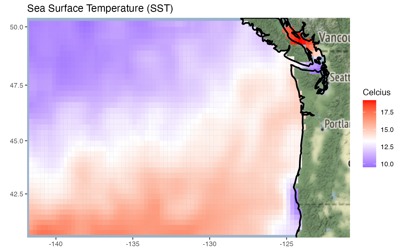

We might want to futz with the look a bit

gg +
  scale_x_continuous(limits = lons, expand = c(-0.01, -0.01)) +
  scale_y_continuous(limits = lats, expand = c(-0.01, -0.01)) +
  theme_bw()

## Scale for 'x' is already present. Adding another scale for 'x', which will
## replace the existing scale.

## Scale for 'y' is already present. Adding another scale for 'y', which will
## replace the existing scale.

3 - Stamen Map

Eli Holmes

2021-08-31

Stamen map the gridded data

Adding a coastline