Part IV. Training on multiple years (bigger than memory)#
Author: Eli Holmes (NOAA)
Now we will put it all together and train on multiple years.
TO DO Get rid of days will lots of NaN in CHL. > 832
Load the libraries#
# Uncomment this line and run if you are in Colab; leave in the !. That is part of the cmd
# !pip install zarr gcsfs xbatcher --quiet
# --- Core data handling libraries ---
import xarray as xr       # for working with labeled multi-dimensional arrays
import numpy as np        # for numerical operations on arrays
import dask.array as da   # for lazy, parallel array operations (used in xarray backends)

# --- Plotting ---
import matplotlib.pyplot as plt  # for creating plots

import xbatcher

# --- TensorFlow setup ---
import os
os.environ['TF_CPP_MIN_LOG_LEVEL'] = '2'  # suppress TensorFlow log spam (0=all, 3=only errors)

import tensorflow as tf  # main deep learning framework

# --- Keras (part of TensorFlow): building and training neural networks ---
from keras.models import Sequential          # lets us stack layers in a simple linear model
from keras.layers import Conv2D              # 2D convolution layer — finds spatial patterns in image-like data
from keras.layers import BatchNormalization  # stabilizes and speeds up training by normalizing activations
from keras.layers import Dropout             # randomly "drops" neurons during training to reduce overfitting
from keras.callbacks import EarlyStopping    # stops training early if validation loss doesn't improve
2025-06-21 02:26:35.210701: E external/local_xla/xla/stream_executor/cuda/cuda_fft.cc:485] Unable to register cuFFT factory: Attempting to register factory for plugin cuFFT when one has already been registered
2025-06-21 02:26:35.228670: E external/local_xla/xla/stream_executor/cuda/cuda_dnn.cc:8454] Unable to register cuDNN factory: Attempting to register factory for plugin cuDNN when one has already been registered
2025-06-21 02:26:35.234116: E external/local_xla/xla/stream_executor/cuda/cuda_blas.cc:1452] Unable to register cuBLAS factory: Attempting to register factory for plugin cuBLAS when one has already been registered
See what machine we are on#
# list all the physical devices
physical_devices = tf.config.list_physical_devices()
print("All Physical Devices:", physical_devices)

# list all the available GPUs
gpus = tf.config.list_physical_devices('GPU')
print("Available GPUs:", gpus)

# Print infomation for available GPU if there exists any
if gpus:
    for gpu in gpus:
        details = tf.config.experimental.get_device_details(gpu)
        print("GPU Details:", details)
else:
    print("No GPU available")
All Physical Devices: [PhysicalDevice(name='/physical_device:CPU:0', device_type='CPU'), PhysicalDevice(name='/physical_device:GPU:0', device_type='GPU')]
Available GPUs: [PhysicalDevice(name='/physical_device:GPU:0', device_type='GPU')]
GPU Details: {'compute_capability': (7, 5), 'device_name': 'Tesla T4'}
Load data#
We definitely need to use open_zarr() so that our data is identified as dask arrays.
# load full dataset 1997 to 2022 from Google bucket
# chunked into 100 day chunks (64, 64 lat/lon)
dataset = xr.open_zarr(
    "gcs://nmfs_odp_nwfsc/CB/mind_the_chl_gap/cnn_tutorial",
    storage_options={"token": "anon"},
    consolidated=True
)
Set up our train, validation and test datasets for xbatcher#
xbatcher requires that we return xarray Datasets, like dataset above, with our input variables (sst, so, etc) and y ready for sending to TensorFlow. We compute the normalization metrics (X_mean X_std) within it and return it for use later (e.g. for validation and test data).
import numpy as np
import dask.array as da
import xarray as xr

def time_series_split_for_xbatcher(
    data, num_var, cat_var=None, split_ratio=(0.7, 0.2, 0.1), seed=42,
    X_mean=None, X_std=None, sample_frac=None
):
    """
    Splits time indices randomly into train/val/test for xbatcher.
    Replaces NaNs, and normalizes numerical variables if mean/std are provided.
    Downsampling happens before normalization so stats match the final training data.

    Parameters:
        data: xarray.Dataset with 'time' dimension
        num_var: list of numerical variable names
        cat_var: list of categorical variable names (no normalization)
        split_ratio: tuple of train, val, test split ratios
        seed: random seed
        X_mean, X_std: optional normalization stats
        sample_frac: optional float (0, 1] to randomly downsample splits

    Returns:
        train_ds, val_ds, test_ds, full_ds: datasets ready for xbatcher
        X_mean, X_std: used for normalization
    """
    if cat_var is None:
        cat_var = []
    output_var = ["y"]

    time_dim = "time"
    if time_dim not in data.dims:
        raise ValueError("Dataset must contain a 'time' dimension.")

    time_len = data.sizes[time_dim]
    rng = np.random.default_rng(seed)
    all_indices = rng.choice(time_len, size=time_len, replace=False)

    train_end = int(split_ratio[0] * time_len)
    val_end = int((split_ratio[0] + split_ratio[1]) * time_len)
    train_idx = np.sort(all_indices[:train_end])
    val_idx = np.sort(all_indices[train_end:val_end])
    test_idx = np.sort(all_indices[val_end:])

    def downsample_idx(idx):
        if sample_frac is not None and len(idx) > 0:
            n_sample = max(1, int(sample_frac * len(idx)))
            return np.sort(rng.choice(idx, size=n_sample, replace=False))
        return idx

    train_idx = downsample_idx(train_idx)
    val_idx = downsample_idx(val_idx)
    test_idx = downsample_idx(test_idx)

    train_data = data.isel(time=train_idx)

    # Compute normalization stats if not provided
    if num_var:
        if X_mean is None or X_std is None:
            stacked = da.stack([train_data[v].data for v in num_var], axis=-1)
            X_mean = da.nanmean(stacked, axis=(0, 1, 2)).compute()
            X_std = da.nanstd(stacked, axis=(0, 1, 2)).compute()
        X_std_safe = da.where(X_std == 0, 1.0, X_std)

    def normalize_and_fill(ds):
        ds_copy = ds.copy()
        for i, var in enumerate(num_var):
            v = (ds[var] - X_mean[i]) / X_std_safe[i]
            ds_copy[var] = xr.DataArray(
                da.nan_to_num(v.data), dims=ds[var].dims, coords=ds[var].coords
            )
        for var in cat_var + output_var:
            ds_copy[var] = xr.DataArray(
                da.nan_to_num(ds[var].data), dims=ds[var].dims, coords=ds[var].coords
            )
        return ds_copy

    train_ds = normalize_and_fill(data.isel(time=train_idx))
    val_ds = normalize_and_fill(data.isel(time=val_idx))
    test_ds = normalize_and_fill(data.isel(time=test_idx))
    full_ds = normalize_and_fill(data)

    return train_ds, val_ds, test_ds, full_ds, X_mean, X_std
Set up train, validation and test years#
I will use different years for each.
# Define variables
input_vars = ["sst", "so", "sin_time", "cos_time", "ocean_mask"]
output_vars = ["y"]
num_var = ["sst", "so"]
cat_var = ["sin_time", "cos_time", "ocean_mask"]
train_yrs = [2015, 2020]
train_years = dataset.sel(time=dataset.time.dt.year.isin(train_yrs))
# Split the dataset using your function
train_ds, _, _, _, X_mean, X_std  = time_series_split_for_xbatcher(
    data=train_years,
    split_ratio=(1.0, 0.0, 0.0),
    num_var=num_var,
    cat_var=cat_var,
    sample_frac = 0.5
)
X_mean
array([301.79614 , 35.002277], dtype=float32)
val_yrs = [2014, 2019]
val_years = dataset.sel(time=dataset.time.dt.year.isin(train_yrs))
_, val_ds, _, _, X_mean, X_std  = time_series_split_for_xbatcher(
    data=train_years,
    split_ratio=(0.0, 1.0, 0.0),
    num_var=num_var,
    cat_var=cat_var,
    sample_frac = 0.25,
    X_mean=X_mean, X_std=X_std
)
Set up xbatcher#
from xbatcher import BatchGenerator

# Use the whole field
input_dims = {"time": 30, "lat": 149, "lon": 181}
input_overlap = {"time": 0, "lat": 0, "lon": 0}

# Create batch generators
train_gen = BatchGenerator(
    train_ds[input_vars + output_vars],
    input_dims=input_dims, input_overlap=input_overlap)
val_gen = BatchGenerator(
    val_ds[input_vars + output_vars],
    input_dims=input_dims, input_overlap=input_overlap)
Set up generator functions to create numpy arrays#
# Generator: yield individual time slices for batches
input_shape = (input_dims["lat"], input_dims["lon"], len(input_vars))
output_shape = (input_dims["lat"], input_dims["lon"], 1)

def train_gen_tf_batches():
    for batch in train_gen:
        time_len = batch["y"].sizes["time"]
        for t in range(time_len):
            x = np.stack([
                batch[var].isel(time=t).data if "time" in batch[var].dims else batch[var].data
                for var in input_vars
            ], axis=-1).astype(np.float32)  # (xx, xx, n_features)
            y = batch["y"].isel(time=t).data[..., np.newaxis].astype(np.float32)  # (xx, xx, 1)
            yield x, y

def val_gen_tf_batches():
    for batch in val_gen:
        time_len = batch["y"].sizes["time"]
        for t in range(time_len):
            x = np.stack([
                batch[var].isel(time=t).data if "time" in batch[var].dims else batch[var].data
                for var in input_vars
            ], axis=-1).astype(np.float32)
            y = batch["y"].isel(time=t).data[..., np.newaxis].astype(np.float32)
            yield x, y


train_dataset_from_gen = tf.data.Dataset.from_generator(
    train_gen_tf_batches,
    output_signature=(
        tf.TensorSpec(shape=input_shape, dtype=tf.float32),
        tf.TensorSpec(shape=output_shape, dtype=tf.float32),
    )
)

val_dataset_from_gen = tf.data.Dataset.from_generator(
    val_gen_tf_batches,
    output_signature=(
        tf.TensorSpec(shape=input_shape, dtype=tf.float32),
        tf.TensorSpec(shape=output_shape, dtype=tf.float32),
    )
)
Final prep of dataset for TensorFlow#
We are not trying to preserve temporal information since we are predicting chlorophyll from same day SST and salinity. So we shuffle() to make sure that everything is i.i.d. for TensorFlow.
shuffle() adds randomness within the training batches
Prevents batch-to-batch correlation
Improves model convergence and generalization
The max shuffle would be the length of the training data per batch up to about 1000-2000. But if the dataset if very large, that would be a lot of overhead and not necessary. In the pper end 10 x number of batches. In our case, the generator yields one sample per time step, so the total training samples ≈ len(train_gen) × input_dims["time"]
print("Number of batches in training set:", len(train_gen))
print("Max shuffle size:", len(train_gen) * input_dims["time"])
Number of batches in training set: 12
Max shuffle size: 360
Using .repeat(). I had to add this when using a generator and specify the training steps per batch. Otherwise, TensorFlow was struggling during the first pass to figure out how much data to use and wasn’t resetting the generator (to give a new set of data) properly.
# you might need to tweak this
BATCH_SIZE = 8
SHUFFLE_N = 100
train_dataset = train_dataset_from_gen.shuffle(SHUFFLE_N).batch(BATCH_SIZE).repeat().prefetch(tf.data.AUTOTUNE)
val_dataset = val_dataset_from_gen.batch(BATCH_SIZE).repeat().prefetch(tf.data.AUTOTUNE)
%%time
# check that shape is (BATCH_SIZE, 149, 181, 5)
for x, y in train_dataset.take(1):
    print("Train x shape:", x.shape)
    print("Train y shape:", y.shape)
Train x shape: (8, 149, 181, 5)
Train y shape: (8, 149, 181, 1)
CPU times: user 3.44 s, sys: 672 ms, total: 4.11 s
Wall time: 6.31 s
Let’s build the model#
We build a simple 3-layer CNN model. Each layer preserves the (lat, lon) shape and learns filters to extract spatial patterns.
from keras.models import Sequential
from keras.layers import Input, Conv2D, BatchNormalization, Dropout

def create_model_CNN(input_shape):
    """
    Create a simple 3-layer CNN model for gridded ocean data.

    Parameters
    ----------
    input_shape : tuple
        The shape of each sample, e.g., (149, 181, 2)

    Returns
    -------
    model : keras.Model
        CNN model to predict CHL from SST and salinity
    """
    model = Sequential()

    # Input layer defines the input dimensions for the CNN
    model.add(Input(shape=input_shape))

    # Layer 1 — learns fine-scale 3x3 spatial features
    # Let the model learn 64 different patterns (filters) in the data at this layer.
    # activation relu is non-linearity
    model.add(Conv2D(filters=64, kernel_size=(3, 3), padding='same', activation='relu'))
    model.add(BatchNormalization())
    model.add(Dropout(0.2))

    # Layer 2 — expands context to 5x5; combines fine features into larger structures
    # Reduce the number of patterns (filters) so we gradually reduce model complexity
    model.add(Conv2D(filters=32, kernel_size=(3, 3), padding='same', activation='relu'))
    model.add(BatchNormalization())
    model.add(Dropout(0.2))

    # Layer 3 — has access to ~7x7 neighborhood; outputs CHL prediction per pixel
    # Combines all the previous layer’s features into a CHL estimate at each pixel
    # 1 response (chl) — hence, 1 prediction pixel = filter
    # linear since predicting a real continuous variable (log CHL)
    model.add(Conv2D(filters=1, kernel_size=(3, 3), padding='same', activation='linear'))

    return model
Let’s train the model#
Because we are working in batches that are chunks of our training set, we only load in a small bit into memory, process that, release the memory and go to the next chunk. This is slow but make sure we can work with larger than memory data.
We load in this 8 × (149 × 181 × n_features + 149 × 181 × 1) × 4 bytes (float32) ≈ a few tens of MB per batch, depending on n_features.
We could do bigger (we have more memory) but this shows the proof of concept.
model = create_model_CNN(input_shape)
model.compile(optimizer='adam', loss='mae', metrics=['mae'])

# Set up early stopping to prevent overfitting
early_stop = EarlyStopping(
    patience=10,              # Stop if validation loss doesn't improve for 10 epochs
    restore_best_weights=True  # Revert to the model weights from the best epoch
)

TRAIN_STEPS_PER_EPOCH = len(train_gen) * input_dims["time"] // BATCH_SIZE
VAL_STEPS_PER_EPOCH = len(val_gen) * input_dims["time"] // BATCH_SIZE

history = model.fit(
    train_dataset,
    epochs=50,                    # Maximum number of training epochs
    steps_per_epoch=TRAIN_STEPS_PER_EPOCH,
    validation_data=val_dataset, # Use validation data during training
    validation_steps=VAL_STEPS_PER_EPOCH,
    callbacks=[early_stop],      # Stop early if no improvement
)
Epoch 1/50
45/45 ━━━━━━━━━━━━━━━━━━━━ 21s 348ms/step - loss: 1.1818 - mae: 1.1818 - val_loss: 0.8262 - val_mae: 0.8262
Epoch 2/50
45/45 ━━━━━━━━━━━━━━━━━━━━ 16s 352ms/step - loss: 0.6575 - mae: 0.6575 - val_loss: 0.6876 - val_mae: 0.6876
Epoch 3/50
45/45 ━━━━━━━━━━━━━━━━━━━━ 16s 361ms/step - loss: 0.3969 - mae: 0.3969 - val_loss: 0.6155 - val_mae: 0.6155
Epoch 4/50
45/45 ━━━━━━━━━━━━━━━━━━━━ 15s 338ms/step - loss: 0.3402 - mae: 0.3402 - val_loss: 0.5467 - val_mae: 0.5467
Epoch 5/50
45/45 ━━━━━━━━━━━━━━━━━━━━ 11s 254ms/step - loss: 0.3211 - mae: 0.3211 - val_loss: 0.4450 - val_mae: 0.4450
Epoch 6/50
45/45 ━━━━━━━━━━━━━━━━━━━━ 15s 289ms/step - loss: 0.3033 - mae: 0.3033 - val_loss: 0.3884 - val_mae: 0.3884
Epoch 7/50
45/45 ━━━━━━━━━━━━━━━━━━━━ 15s 232ms/step - loss: 0.2892 - mae: 0.2892 - val_loss: 0.3564 - val_mae: 0.3564
Epoch 8/50
45/45 ━━━━━━━━━━━━━━━━━━━━ 15s 232ms/step - loss: 0.2771 - mae: 0.2771 - val_loss: 0.3057 - val_mae: 0.3057
Epoch 9/50
45/45 ━━━━━━━━━━━━━━━━━━━━ 15s 233ms/step - loss: 0.2695 - mae: 0.2695 - val_loss: 0.2768 - val_mae: 0.2768
Epoch 10/50
45/45 ━━━━━━━━━━━━━━━━━━━━ 14s 207ms/step - loss: 0.2636 - mae: 0.2636 - val_loss: 0.2634 - val_mae: 0.2634
Epoch 11/50
45/45 ━━━━━━━━━━━━━━━━━━━━ 15s 234ms/step - loss: 0.2631 - mae: 0.2631 - val_loss: 0.2325 - val_mae: 0.2325
Epoch 12/50
45/45 ━━━━━━━━━━━━━━━━━━━━ 15s 227ms/step - loss: 0.2597 - mae: 0.2597 - val_loss: 0.2200 - val_mae: 0.2200
Epoch 13/50
45/45 ━━━━━━━━━━━━━━━━━━━━ 15s 230ms/step - loss: 0.2524 - mae: 0.2524 - val_loss: 0.2109 - val_mae: 0.2109
Epoch 14/50
45/45 ━━━━━━━━━━━━━━━━━━━━ 15s 234ms/step - loss: 0.2475 - mae: 0.2475 - val_loss: 0.2151 - val_mae: 0.2151
Epoch 15/50
45/45 ━━━━━━━━━━━━━━━━━━━━ 14s 218ms/step - loss: 0.2454 - mae: 0.2454 - val_loss: 0.2022 - val_mae: 0.2022
Epoch 16/50
45/45 ━━━━━━━━━━━━━━━━━━━━ 15s 234ms/step - loss: 0.2395 - mae: 0.2395 - val_loss: 0.2020 - val_mae: 0.2020
Epoch 17/50
45/45 ━━━━━━━━━━━━━━━━━━━━ 15s 238ms/step - loss: 0.2360 - mae: 0.2360 - val_loss: 0.2106 - val_mae: 0.2106
Epoch 18/50
45/45 ━━━━━━━━━━━━━━━━━━━━ 14s 208ms/step - loss: 0.2439 - mae: 0.2439 - val_loss: 0.2219 - val_mae: 0.2219
Epoch 19/50
45/45 ━━━━━━━━━━━━━━━━━━━━ 15s 224ms/step - loss: 0.2451 - mae: 0.2451 - val_loss: 0.2152 - val_mae: 0.2152
Epoch 20/50
45/45 ━━━━━━━━━━━━━━━━━━━━ 15s 224ms/step - loss: 0.2397 - mae: 0.2397 - val_loss: 0.2036 - val_mae: 0.2036
Epoch 21/50
45/45 ━━━━━━━━━━━━━━━━━━━━ 15s 235ms/step - loss: 0.2398 - mae: 0.2398 - val_loss: 0.2078 - val_mae: 0.2078
Epoch 22/50
45/45 ━━━━━━━━━━━━━━━━━━━━ 14s 207ms/step - loss: 0.2484 - mae: 0.2484 - val_loss: 0.2060 - val_mae: 0.2060
Epoch 23/50
45/45 ━━━━━━━━━━━━━━━━━━━━ 15s 231ms/step - loss: 0.2378 - mae: 0.2378 - val_loss: 0.2074 - val_mae: 0.2074
Epoch 24/50
45/45 ━━━━━━━━━━━━━━━━━━━━ 15s 227ms/step - loss: 0.2311 - mae: 0.2311 - val_loss: 0.2094 - val_mae: 0.2094
Epoch 25/50
45/45 ━━━━━━━━━━━━━━━━━━━━ 15s 228ms/step - loss: 0.2322 - mae: 0.2322 - val_loss: 0.2039 - val_mae: 0.2039
Epoch 26/50
45/45 ━━━━━━━━━━━━━━━━━━━━ 14s 210ms/step - loss: 0.2391 - mae: 0.2391 - val_loss: 0.2016 - val_mae: 0.2016
Epoch 27/50
45/45 ━━━━━━━━━━━━━━━━━━━━ 15s 237ms/step - loss: 0.2369 - mae: 0.2369 - val_loss: 0.2013 - val_mae: 0.2013
Epoch 28/50
45/45 ━━━━━━━━━━━━━━━━━━━━ 15s 234ms/step - loss: 0.2272 - mae: 0.2272 - val_loss: 0.1952 - val_mae: 0.1952
Epoch 29/50
45/45 ━━━━━━━━━━━━━━━━━━━━ 15s 225ms/step - loss: 0.2326 - mae: 0.2326 - val_loss: 0.2030 - val_mae: 0.2030
Epoch 30/50
45/45 ━━━━━━━━━━━━━━━━━━━━ 14s 208ms/step - loss: 0.2278 - mae: 0.2278 - val_loss: 0.1981 - val_mae: 0.1981
Epoch 31/50
45/45 ━━━━━━━━━━━━━━━━━━━━ 15s 226ms/step - loss: 0.2233 - mae: 0.2233 - val_loss: 0.2055 - val_mae: 0.2055
Epoch 32/50
45/45 ━━━━━━━━━━━━━━━━━━━━ 15s 236ms/step - loss: 0.2325 - mae: 0.2325 - val_loss: 0.2021 - val_mae: 0.2021
Epoch 33/50
45/45 ━━━━━━━━━━━━━━━━━━━━ 14s 219ms/step - loss: 0.2266 - mae: 0.2266 - val_loss: 0.1996 - val_mae: 0.1996
Epoch 34/50
45/45 ━━━━━━━━━━━━━━━━━━━━ 15s 233ms/step - loss: 0.2317 - mae: 0.2317 - val_loss: 0.1962 - val_mae: 0.1962
Epoch 35/50
45/45 ━━━━━━━━━━━━━━━━━━━━ 15s 228ms/step - loss: 0.2351 - mae: 0.2351 - val_loss: 0.2037 - val_mae: 0.2037
Epoch 36/50
45/45 ━━━━━━━━━━━━━━━━━━━━ 15s 228ms/step - loss: 0.2371 - mae: 0.2371 - val_loss: 0.1977 - val_mae: 0.1977
Epoch 37/50
45/45 ━━━━━━━━━━━━━━━━━━━━ 15s 228ms/step - loss: 0.2247 - mae: 0.2247 - val_loss: 0.1974 - val_mae: 0.1974
Epoch 38/50
45/45 ━━━━━━━━━━━━━━━━━━━━ 14s 217ms/step - loss: 0.2233 - mae: 0.2233 - val_loss: 0.1988 - val_mae: 0.1988
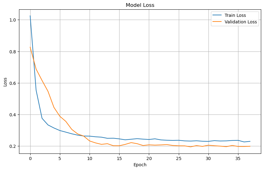
Plot training & validation loss values#
plt.figure(figsize=(10, 6))
plt.plot(history.history['loss'], label='Train Loss')
plt.plot(history.history['val_loss'], label='Validation Loss')
plt.title('Model Loss')
plt.xlabel('Epoch')
plt.ylabel('Loss')
plt.legend(loc='upper right')
plt.grid(True)
plt.show()
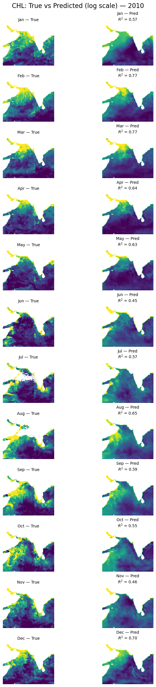
Plot all months#
import numpy as np
import pandas as pd
import matplotlib.pyplot as plt

def plot_true_vs_predicted(data, year, model, X_mean, X_std, num_var, cat_var):
    """
    Plot true vs predicted output for first available day of each month in data_test.

    Parameters:
        data (xarray.Dataset): Contains variables 'y', 'ocean_mask', and coords 'lat', 'lon', 'time'
        year (string in format XXXX): The year to use.
        model (tf.keras.Model): Trained model with a .predict() method
        X_mean (np.ndarray): mean from the model training data (num_vars only)
        X_std (np.ndarray): std from the model training data
        num_var (np.ndarry): The variables to be standardized with `X_mean` and `X_std`
        cat_var (np.ndarry): The variables to be included in X, y but not standardized.
    """
    # Split the dataset to get full_ds
    _, _, _, year_ds, _, _ = time_series_split_for_xbatcher(
        data=data.sel(time=year),
        num_var=num_var,
        cat_var=cat_var,
        X_mean=X_mean,
        X_std=X_std,
    )

    # Get available time points and group by month
    available_dates = pd.to_datetime(year_ds.time.values)
    monthly_dates = (
        pd.Series(available_dates)
        .groupby([available_dates.year, available_dates.month])
        .min()
        .sort_values()
    )
    n_months = len(monthly_dates)

    # lat/lon info
    lat = year_ds.lat.values
    lon = year_ds.lon.values
    extent = [lon.min(), lon.max(), lat.min(), lat.max()]
    flip_lat = lat[0] > lat[-1]
    land_mask = ~year_ds["ocean_mask"].values.astype(bool)

    # Create figure and axes
    fig, axs = plt.subplots(n_months, 2, figsize=(7, 2 * n_months), constrained_layout=True)

    for i, date in enumerate(monthly_dates):
        # Select dataset for this date
        ds_at_time = year_ds.sel(time=np.datetime64(date))

        # Prepare model input: stack input variables into (lat, lon, n_features)
        input_data = np.stack([
            ds_at_time[var].values for var in input_vars
        ], axis=-1)

        # Predict: shape (lat, lon)
        predicted_output = model.predict(input_data[np.newaxis, ...])[0, ..., 0]

        # True output
        true_output = data["y"].sel(time=np.datetime64(date)).values

        # Mask land
        predicted_output[land_mask] = np.nan
        true_output[land_mask] = np.nan

        # Flip latitude if needed
        if flip_lat:
            true_output = np.flipud(true_output)
            predicted_output = np.flipud(predicted_output)

        # Shared color scale
        vmin = np.nanpercentile([true_output, predicted_output], 5)
        vmax = np.nanpercentile([true_output, predicted_output], 95)

        # Compute R²
        from sklearn.metrics import r2_score
        true_flat = true_output.flatten()
        pred_flat = predicted_output.flatten()
        valid_mask = ~np.isnan(true_flat) & ~np.isnan(pred_flat)
        r2 = r2_score(true_flat[valid_mask], pred_flat[valid_mask])

        # Plot true
        axs[i, 0].imshow(true_output, origin='lower', extent=extent,
                         vmin=vmin, vmax=vmax, cmap='viridis',
                         aspect='equal')
        axs[i, 0].set_title(f"{date.strftime('%b')} — True", fontsize=10)
        axs[i, 0].axis('off')

        # Plot predicted with R²
        axs[i, 1].imshow(predicted_output, origin='lower', extent=extent,
                         vmin=vmin, vmax=vmax, cmap='viridis',
                         aspect='equal')
        axs[i, 1].set_title(f"{date.strftime('%b')} — Pred\n$R^2$ = {r2:.2f}", fontsize=10)
        axs[i, 1].axis('off')

    plt.suptitle(f'CHL: True vs Predicted (log scale) — {year}', fontsize=16)
    plt.show()
plot_true_vs_predicted(dataset, "2010", model, X_mean, X_std, num_var, cat_var)
1/1 ━━━━━━━━━━━━━━━━━━━━ 0s 298ms/step
1/1 ━━━━━━━━━━━━━━━━━━━━ 0s 18ms/step
1/1 ━━━━━━━━━━━━━━━━━━━━ 0s 18ms/step
1/1 ━━━━━━━━━━━━━━━━━━━━ 0s 19ms/step
1/1 ━━━━━━━━━━━━━━━━━━━━ 0s 19ms/step
1/1 ━━━━━━━━━━━━━━━━━━━━ 0s 18ms/step
1/1 ━━━━━━━━━━━━━━━━━━━━ 0s 18ms/step
1/1 ━━━━━━━━━━━━━━━━━━━━ 0s 18ms/step
1/1 ━━━━━━━━━━━━━━━━━━━━ 0s 18ms/step
1/1 ━━━━━━━━━━━━━━━━━━━━ 0s 18ms/step
1/1 ━━━━━━━━━━━━━━━━━━━━ 0s 18ms/step
1/1 ━━━━━━━━━━━━━━━━━━━━ 0s 18ms/step
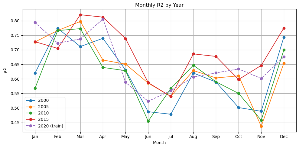
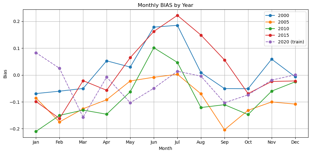
Comparing fits with metrics#
import matplotlib.pyplot as plt
import numpy as np
import pandas as pd
from sklearn.metrics import r2_score, mean_absolute_error
import calendar

def plot_metric_by_month(data, years, model, X_mean, X_std, num_var, cat_var,
                         training_year=None, metric='r2'):
    """
    Plot a selected evaluation metric (R², RMSE, MAE, or Bias) by month for each year.

    Parameters:
        data (xarray.Dataset): Contains 'y', predictors, and coordinates
        years (list of str): Years to evaluate, e.g., ['2018', '2019', '2020']
        model (tf.keras.Model): Trained model with .predict() method
        X_mean, X_std (np.ndarray): Normalization stats for num_vars
        num_var, cat_var (list of str): Variable names
        training_year (str, optional): If specified, highlights that year specially
        metric (str): One of ['r2', 'rmse', 'mae', 'bias']
    """
    assert metric in ['r2', 'rmse', 'mae', 'bias'], "Invalid metric. Choose from 'r2', 'rmse', 'mae', 'bias'."

    metric_by_year_month = {}

    for year in years:
        data_year = data.sel(time=year)
        dates = pd.to_datetime(data_year.time.values)

        monthly_dates = (
            pd.Series(dates)
            .groupby([dates.year, dates.month])
            .min()
            .sort_values()
        )

        _, _, _, year_ds, _, _ = time_series_split_for_xbatcher(
            data=data.sel(time=year),
            num_var=num_var,
            cat_var=cat_var,
            X_mean=X_mean,
            X_std=X_std,
            )

        metric_scores = []
        for date in monthly_dates:
            idx = np.where(dates == date)[0][0]
            true_output = data_year['y'].sel(time=date).values
            ds_at_time = year_ds.sel(time=np.datetime64(date))
            pred_input = np.stack([
                ds_at_time[var].values for var in input_vars
            ], axis=-1)

            pred_output = model.predict(pred_input[np.newaxis, ...], verbose=0)[0][:, :, 0]
            pred_output[data_year["ocean_mask"].values == 0.0] = np.nan

            mask = ~np.isnan(true_output) & ~np.isnan(pred_output)
            y_true = true_output[mask].flatten()
            y_pred = pred_output[mask].flatten()

            if metric == 'r2':
                score = r2_score(y_true, y_pred)
            elif metric == 'rmse':
                score = np.sqrt(np.mean((y_true - y_pred)**2))
            elif metric == 'mae':
                score = mean_absolute_error(y_true, y_pred)
            elif metric == 'bias':
                score = np.mean(y_pred - y_true)

            metric_scores.append(score)

        metric_by_year_month[year] = (monthly_dates.dt.month.values, metric_scores)

    # Plotting
    plt.figure(figsize=(10, 5))
    for year, (months, scores) in metric_by_year_month.items():
        label = f"{year} (train)" if year == training_year else year
        style = "--" if year == training_year else "-"
        plt.plot(months, scores, style, marker='o', label=label)

    plt.xlabel("Month")
    plt.ylabel({
        'r2': "$R^2$",
        'rmse': "RMSE",
        'mae': "MAE",
        'bias': "Bias"
    }[metric])
    plt.title(f"Monthly {metric.upper()} by Year")
    plt.xticks(np.arange(1, 13), calendar.month_abbr[1:13])
    plt.legend()
    plt.grid(True)
    plt.tight_layout()
    plt.show()
%%time
plot_metric_by_month(dataset, ['2000', '2005', '2010', '2015', '2020'], model, X_mean, X_std, num_var, cat_var, training_year="2020")
%%time
plot_metric_by_month(dataset, ['2000', '2005', '2010', '2015', '2020'], model,
                     X_mean, X_std, num_var, cat_var, training_year="2020", metric="bias")
CPU times: user 17.2 s, sys: 2.22 s, total: 19.4 s
Wall time: 38.8 s
Summary#
That concludes the series on 2D CNNs for predicting chlorophyll in a region.
train_ds.time.values
array(['2015-01-01T00:00:00.000000000', '2015-01-03T00:00:00.000000000',
       '2015-01-05T00:00:00.000000000', '2015-01-07T00:00:00.000000000',
       '2015-01-08T00:00:00.000000000', '2015-01-09T00:00:00.000000000',
       '2015-01-10T00:00:00.000000000', '2015-01-11T00:00:00.000000000',
       '2015-01-12T00:00:00.000000000', '2015-01-14T00:00:00.000000000',
       '2015-01-15T00:00:00.000000000', '2015-01-16T00:00:00.000000000',
       '2015-01-17T00:00:00.000000000', '2015-01-18T00:00:00.000000000',
       '2015-01-19T00:00:00.000000000', '2015-01-21T00:00:00.000000000',
       '2015-01-23T00:00:00.000000000', '2015-01-28T00:00:00.000000000',
       '2015-01-30T00:00:00.000000000', '2015-02-01T00:00:00.000000000',
       '2015-02-02T00:00:00.000000000', '2015-02-07T00:00:00.000000000',
       '2015-02-08T00:00:00.000000000', '2015-02-09T00:00:00.000000000',
       '2015-02-10T00:00:00.000000000', '2015-02-11T00:00:00.000000000',
       '2015-02-13T00:00:00.000000000', '2015-02-15T00:00:00.000000000',
       '2015-02-19T00:00:00.000000000', '2015-02-24T00:00:00.000000000',
       '2015-02-25T00:00:00.000000000', '2015-02-26T00:00:00.000000000',
       '2015-02-28T00:00:00.000000000', '2015-03-01T00:00:00.000000000',
       '2015-03-05T00:00:00.000000000', '2015-03-06T00:00:00.000000000',
       '2015-03-07T00:00:00.000000000', '2015-03-08T00:00:00.000000000',
       '2015-03-10T00:00:00.000000000', '2015-03-13T00:00:00.000000000',
       '2015-03-14T00:00:00.000000000', '2015-03-16T00:00:00.000000000',
       '2015-03-17T00:00:00.000000000', '2015-03-20T00:00:00.000000000',
       '2015-03-21T00:00:00.000000000', '2015-03-24T00:00:00.000000000',
       '2015-03-25T00:00:00.000000000', '2015-03-29T00:00:00.000000000',
       '2015-03-30T00:00:00.000000000', '2015-03-31T00:00:00.000000000',
       '2015-04-01T00:00:00.000000000', '2015-04-04T00:00:00.000000000',
       '2015-04-06T00:00:00.000000000', '2015-04-07T00:00:00.000000000',
       '2015-04-09T00:00:00.000000000', '2015-04-10T00:00:00.000000000',
       '2015-04-14T00:00:00.000000000', '2015-04-15T00:00:00.000000000',
       '2015-04-16T00:00:00.000000000', '2015-04-17T00:00:00.000000000',
       '2015-04-19T00:00:00.000000000', '2015-04-20T00:00:00.000000000',
       '2015-04-22T00:00:00.000000000', '2015-04-23T00:00:00.000000000',
       '2015-04-26T00:00:00.000000000', '2015-04-27T00:00:00.000000000',
       '2015-04-29T00:00:00.000000000', '2015-05-02T00:00:00.000000000',
       '2015-05-09T00:00:00.000000000', '2015-05-10T00:00:00.000000000',
       '2015-05-11T00:00:00.000000000', '2015-05-13T00:00:00.000000000',
       '2015-05-14T00:00:00.000000000', '2015-05-16T00:00:00.000000000',
       '2015-05-17T00:00:00.000000000', '2015-05-18T00:00:00.000000000',
       '2015-05-19T00:00:00.000000000', '2015-05-20T00:00:00.000000000',
       '2015-05-22T00:00:00.000000000', '2015-05-24T00:00:00.000000000',
       '2015-05-25T00:00:00.000000000', '2015-05-30T00:00:00.000000000',
       '2015-06-01T00:00:00.000000000', '2015-06-02T00:00:00.000000000',
       '2015-06-03T00:00:00.000000000', '2015-06-04T00:00:00.000000000',
       '2015-06-06T00:00:00.000000000', '2015-06-10T00:00:00.000000000',
       '2015-06-11T00:00:00.000000000', '2015-06-12T00:00:00.000000000',
       '2015-06-14T00:00:00.000000000', '2015-06-18T00:00:00.000000000',
       '2015-06-19T00:00:00.000000000', '2015-06-20T00:00:00.000000000',
       '2015-06-22T00:00:00.000000000', '2015-06-23T00:00:00.000000000',
       '2015-06-25T00:00:00.000000000', '2015-07-02T00:00:00.000000000',
       '2015-07-04T00:00:00.000000000', '2015-07-07T00:00:00.000000000',
       '2015-07-09T00:00:00.000000000', '2015-07-11T00:00:00.000000000',
       '2015-07-14T00:00:00.000000000', '2015-07-16T00:00:00.000000000',
       '2015-07-18T00:00:00.000000000', '2015-07-21T00:00:00.000000000',
       '2015-07-22T00:00:00.000000000', '2015-07-24T00:00:00.000000000',
       '2015-07-27T00:00:00.000000000', '2015-07-30T00:00:00.000000000',
       '2015-07-31T00:00:00.000000000', '2015-08-01T00:00:00.000000000',
       '2015-08-03T00:00:00.000000000', '2015-08-04T00:00:00.000000000',
       '2015-08-06T00:00:00.000000000', '2015-08-08T00:00:00.000000000',
       '2015-08-11T00:00:00.000000000', '2015-08-13T00:00:00.000000000',
       '2015-08-15T00:00:00.000000000', '2015-08-16T00:00:00.000000000',
       '2015-08-17T00:00:00.000000000', '2015-08-19T00:00:00.000000000',
       '2015-08-22T00:00:00.000000000', '2015-08-25T00:00:00.000000000',
       '2015-08-26T00:00:00.000000000', '2015-08-29T00:00:00.000000000',
       '2015-08-31T00:00:00.000000000', '2015-09-02T00:00:00.000000000',
       '2015-09-03T00:00:00.000000000', '2015-09-04T00:00:00.000000000',
       '2015-09-10T00:00:00.000000000', '2015-09-11T00:00:00.000000000',
       '2015-09-13T00:00:00.000000000', '2015-09-14T00:00:00.000000000',
       '2015-09-16T00:00:00.000000000', '2015-09-18T00:00:00.000000000',
       '2015-09-20T00:00:00.000000000', '2015-09-21T00:00:00.000000000',
       '2015-09-22T00:00:00.000000000', '2015-09-23T00:00:00.000000000',
       '2015-09-24T00:00:00.000000000', '2015-09-25T00:00:00.000000000',
       '2015-10-01T00:00:00.000000000', '2015-10-04T00:00:00.000000000',
       '2015-10-06T00:00:00.000000000', '2015-10-10T00:00:00.000000000',
       '2015-10-12T00:00:00.000000000', '2015-10-14T00:00:00.000000000',
       '2015-10-17T00:00:00.000000000', '2015-10-18T00:00:00.000000000',
       '2015-10-19T00:00:00.000000000', '2015-10-21T00:00:00.000000000',
       '2015-10-23T00:00:00.000000000', '2015-10-27T00:00:00.000000000',
       '2015-10-29T00:00:00.000000000', '2015-11-01T00:00:00.000000000',
       '2015-11-02T00:00:00.000000000', '2015-11-03T00:00:00.000000000',
       '2015-11-04T00:00:00.000000000', '2015-11-08T00:00:00.000000000',
       '2015-11-09T00:00:00.000000000', '2015-11-11T00:00:00.000000000',
       '2015-11-12T00:00:00.000000000', '2015-11-13T00:00:00.000000000',
       '2015-11-19T00:00:00.000000000', '2015-11-20T00:00:00.000000000',
       '2015-11-24T00:00:00.000000000', '2015-11-25T00:00:00.000000000',
       '2015-11-28T00:00:00.000000000', '2015-11-30T00:00:00.000000000',
       '2015-12-02T00:00:00.000000000', '2015-12-03T00:00:00.000000000',
       '2015-12-04T00:00:00.000000000', '2015-12-05T00:00:00.000000000',
       '2015-12-06T00:00:00.000000000', '2015-12-08T00:00:00.000000000',
       '2015-12-10T00:00:00.000000000', '2015-12-13T00:00:00.000000000',
       '2015-12-14T00:00:00.000000000', '2015-12-18T00:00:00.000000000',
       '2015-12-23T00:00:00.000000000', '2015-12-25T00:00:00.000000000',
       '2015-12-27T00:00:00.000000000', '2015-12-28T00:00:00.000000000',
       '2020-01-01T00:00:00.000000000', '2020-01-03T00:00:00.000000000',
       '2020-01-04T00:00:00.000000000', '2020-01-08T00:00:00.000000000',
       '2020-01-11T00:00:00.000000000', '2020-01-13T00:00:00.000000000',
       '2020-01-15T00:00:00.000000000', '2020-01-17T00:00:00.000000000',
       '2020-01-21T00:00:00.000000000', '2020-01-22T00:00:00.000000000',
       '2020-01-24T00:00:00.000000000', '2020-01-26T00:00:00.000000000',
       '2020-01-27T00:00:00.000000000', '2020-01-28T00:00:00.000000000',
       '2020-01-29T00:00:00.000000000', '2020-01-30T00:00:00.000000000',
       '2020-02-03T00:00:00.000000000', '2020-02-05T00:00:00.000000000',
       '2020-02-06T00:00:00.000000000', '2020-02-07T00:00:00.000000000',
       '2020-02-08T00:00:00.000000000', '2020-02-09T00:00:00.000000000',
       '2020-02-10T00:00:00.000000000', '2020-02-12T00:00:00.000000000',
       '2020-02-14T00:00:00.000000000', '2020-02-15T00:00:00.000000000',
       '2020-02-19T00:00:00.000000000', '2020-02-20T00:00:00.000000000',
       '2020-02-21T00:00:00.000000000', '2020-02-23T00:00:00.000000000',
       '2020-02-25T00:00:00.000000000', '2020-03-02T00:00:00.000000000',
       '2020-03-06T00:00:00.000000000', '2020-03-07T00:00:00.000000000',
       '2020-03-08T00:00:00.000000000', '2020-03-15T00:00:00.000000000',
       '2020-03-16T00:00:00.000000000', '2020-03-22T00:00:00.000000000',
       '2020-03-24T00:00:00.000000000', '2020-03-28T00:00:00.000000000',
       '2020-03-30T00:00:00.000000000', '2020-03-31T00:00:00.000000000',
       '2020-04-02T00:00:00.000000000', '2020-04-04T00:00:00.000000000',
       '2020-04-05T00:00:00.000000000', '2020-04-06T00:00:00.000000000',
       '2020-04-07T00:00:00.000000000', '2020-04-08T00:00:00.000000000',
       '2020-04-09T00:00:00.000000000', '2020-04-10T00:00:00.000000000',
       '2020-04-13T00:00:00.000000000', '2020-04-14T00:00:00.000000000',
       '2020-04-16T00:00:00.000000000', '2020-04-19T00:00:00.000000000',
       '2020-04-20T00:00:00.000000000', '2020-04-22T00:00:00.000000000',
       '2020-04-24T00:00:00.000000000', '2020-04-26T00:00:00.000000000',
       '2020-04-27T00:00:00.000000000', '2020-04-29T00:00:00.000000000',
       '2020-04-30T00:00:00.000000000', '2020-05-03T00:00:00.000000000',
       '2020-05-07T00:00:00.000000000', '2020-05-09T00:00:00.000000000',
       '2020-05-11T00:00:00.000000000', '2020-05-12T00:00:00.000000000',
       '2020-05-15T00:00:00.000000000', '2020-05-17T00:00:00.000000000',
       '2020-05-18T00:00:00.000000000', '2020-05-19T00:00:00.000000000',
       '2020-05-20T00:00:00.000000000', '2020-05-25T00:00:00.000000000',
       '2020-05-27T00:00:00.000000000', '2020-06-03T00:00:00.000000000',
       '2020-06-05T00:00:00.000000000', '2020-06-06T00:00:00.000000000',
       '2020-06-07T00:00:00.000000000', '2020-06-08T00:00:00.000000000',
       '2020-06-09T00:00:00.000000000', '2020-06-10T00:00:00.000000000',
       '2020-06-11T00:00:00.000000000', '2020-06-12T00:00:00.000000000',
       '2020-06-13T00:00:00.000000000', '2020-06-16T00:00:00.000000000',
       '2020-06-17T00:00:00.000000000', '2020-06-19T00:00:00.000000000',
       '2020-06-20T00:00:00.000000000', '2020-06-22T00:00:00.000000000',
       '2020-06-24T00:00:00.000000000', '2020-06-26T00:00:00.000000000',
       '2020-06-27T00:00:00.000000000', '2020-06-28T00:00:00.000000000',
       '2020-06-30T00:00:00.000000000', '2020-07-02T00:00:00.000000000',
       '2020-07-05T00:00:00.000000000', '2020-07-06T00:00:00.000000000',
       '2020-07-07T00:00:00.000000000', '2020-07-10T00:00:00.000000000',
       '2020-07-12T00:00:00.000000000', '2020-07-14T00:00:00.000000000',
       '2020-07-16T00:00:00.000000000', '2020-07-18T00:00:00.000000000',
       '2020-07-19T00:00:00.000000000', '2020-07-20T00:00:00.000000000',
       '2020-07-22T00:00:00.000000000', '2020-07-23T00:00:00.000000000',
       '2020-07-26T00:00:00.000000000', '2020-07-30T00:00:00.000000000',
       '2020-07-31T00:00:00.000000000', '2020-08-02T00:00:00.000000000',
       '2020-08-05T00:00:00.000000000', '2020-08-06T00:00:00.000000000',
       '2020-08-07T00:00:00.000000000', '2020-08-11T00:00:00.000000000',
       '2020-08-12T00:00:00.000000000', '2020-08-13T00:00:00.000000000',
       '2020-08-14T00:00:00.000000000', '2020-08-21T00:00:00.000000000',
       '2020-08-22T00:00:00.000000000', '2020-08-24T00:00:00.000000000',
       '2020-08-25T00:00:00.000000000', '2020-08-26T00:00:00.000000000',
       '2020-08-28T00:00:00.000000000', '2020-08-29T00:00:00.000000000',
       '2020-08-30T00:00:00.000000000', '2020-08-31T00:00:00.000000000',
       '2020-09-01T00:00:00.000000000', '2020-09-03T00:00:00.000000000',
       '2020-09-06T00:00:00.000000000', '2020-09-08T00:00:00.000000000',
       '2020-09-09T00:00:00.000000000', '2020-09-10T00:00:00.000000000',
       '2020-09-12T00:00:00.000000000', '2020-09-13T00:00:00.000000000',
       '2020-09-20T00:00:00.000000000', '2020-09-26T00:00:00.000000000',
       '2020-09-29T00:00:00.000000000', '2020-09-30T00:00:00.000000000',
       '2020-10-01T00:00:00.000000000', '2020-10-02T00:00:00.000000000',
       '2020-10-03T00:00:00.000000000', '2020-10-04T00:00:00.000000000',
       '2020-10-05T00:00:00.000000000', '2020-10-06T00:00:00.000000000',
       '2020-10-07T00:00:00.000000000', '2020-10-14T00:00:00.000000000',
       '2020-10-16T00:00:00.000000000', '2020-10-19T00:00:00.000000000',
       '2020-10-20T00:00:00.000000000', '2020-10-21T00:00:00.000000000',
       '2020-10-22T00:00:00.000000000', '2020-10-23T00:00:00.000000000',
       '2020-10-27T00:00:00.000000000', '2020-10-28T00:00:00.000000000',
       '2020-11-01T00:00:00.000000000', '2020-11-02T00:00:00.000000000',
       '2020-11-04T00:00:00.000000000', '2020-11-06T00:00:00.000000000',
       '2020-11-09T00:00:00.000000000', '2020-11-12T00:00:00.000000000',
       '2020-11-13T00:00:00.000000000', '2020-11-15T00:00:00.000000000',
       '2020-11-16T00:00:00.000000000', '2020-11-17T00:00:00.000000000',
       '2020-11-24T00:00:00.000000000', '2020-11-26T00:00:00.000000000',
       '2020-11-28T00:00:00.000000000', '2020-11-30T00:00:00.000000000',
       '2020-12-03T00:00:00.000000000', '2020-12-04T00:00:00.000000000',
       '2020-12-06T00:00:00.000000000', '2020-12-08T00:00:00.000000000',
       '2020-12-11T00:00:00.000000000', '2020-12-12T00:00:00.000000000',
       '2020-12-13T00:00:00.000000000', '2020-12-15T00:00:00.000000000',
       '2020-12-18T00:00:00.000000000', '2020-12-26T00:00:00.000000000',
       '2020-12-28T00:00:00.000000000', '2020-12-30T00:00:00.000000000',
       '2020-12-31T00:00:00.000000000'], dtype='datetime64[ns]')