Loading and Working with the Dataset#
This notebook is based on an original notebook by Minh Phan (UW Varanasi intern 2023). It describes how to read and work with the Indian Ocean dataset.
The dataset contains chlorophyl concentrations, atmospheric and oceanographic fields used to force the machine learning models. The dataset is a single zarr file.
Note
cmocean is problematic to import. If the import step fails, uncomment the cell below and run it to pip install the package. You can uncomment both lines by highlighting both lines and ctrl-/.
# %%capture
# %pip install cmocean
import xarray as xr
import numpy as np
import pandas as pd
import matplotlib.pyplot as plt # simple plotting
import holoviews as hv # simple plotting
import hvplot.xarray # simple plotting
import cmocean
Read data#
xarray can be used to open zarr files.
ds = xr.open_zarr("~/shared/mind_the_chl_gap/IO.zarr")
The dataset representation can viewed below. Clicking on Data variables displays the full list of variables.
ds
<xarray.Dataset> Size: 66GB
Dimensions:                       (time: 16071, lat: 177, lon: 241)
Coordinates:
  * lat                           (lat) float32 708B 32.0 31.75 ... -11.75 -12.0
  * lon                           (lon) float32 964B 42.0 42.25 ... 101.8 102.0
  * time                          (time) datetime64[ns] 129kB 1979-01-01 ... ...
Data variables: (12/27)
    CHL                           (time, lat, lon) float32 3GB dask.array<chunksize=(100, 177, 241), meta=np.ndarray>
    CHL_cmes-cloud                (time, lat, lon) uint8 686MB dask.array<chunksize=(100, 177, 241), meta=np.ndarray>
    CHL_cmes-gapfree              (time, lat, lon) float32 3GB dask.array<chunksize=(100, 177, 241), meta=np.ndarray>
    CHL_cmes-land                 (lat, lon) uint8 43kB dask.array<chunksize=(177, 241), meta=np.ndarray>
    CHL_cmes-level3               (time, lat, lon) float32 3GB dask.array<chunksize=(100, 177, 241), meta=np.ndarray>
    CHL_cmes_flags-gapfree        (time, lat, lon) float32 3GB dask.array<chunksize=(100, 177, 241), meta=np.ndarray>
    ...                            ...
    ug_curr                       (time, lat, lon) float32 3GB dask.array<chunksize=(100, 177, 241), meta=np.ndarray>
    v_curr                        (time, lat, lon) float32 3GB dask.array<chunksize=(100, 177, 241), meta=np.ndarray>
    v_wind                        (time, lat, lon) float32 3GB dask.array<chunksize=(100, 177, 241), meta=np.ndarray>
    vg_curr                       (time, lat, lon) float32 3GB dask.array<chunksize=(100, 177, 241), meta=np.ndarray>
    wind_dir                      (time, lat, lon) float32 3GB dask.array<chunksize=(100, 177, 241), meta=np.ndarray>
    wind_speed                    (time, lat, lon) float32 3GB dask.array<chunksize=(100, 177, 241), meta=np.ndarray>
Attributes: (12/92)
    Conventions:                     CF-1.8, ACDD-1.3
    DPM_reference:                   GC-UD-ACRI-PUG
    IODD_reference:                  GC-UD-ACRI-PUG
    acknowledgement:                 The Licensees will ensure that original ...
    citation:                        The Licensees will ensure that original ...
    cmems_product_id:                OCEANCOLOUR_GLO_BGC_L3_MY_009_103
    ...                              ...
    time_coverage_end:               2024-04-18T02:58:23Z
    time_coverage_resolution:        P1D
    time_coverage_start:             2024-04-16T21:12:05Z
    title:                           cmems_obs-oc_glo_bgc-plankton_my_l3-mult...
    westernmost_longitude:           -180.0
westernmost_valid_longitude: -180.0- time: 16071
- lat: 177
- lon: 241
- lat(lat)float3232.0 31.75 31.5 ... -11.75 -12.0
- long_name :
- latitude
- standard_name :
- latitude
- units :
- degrees_north
array([ 32. , 31.75, 31.5 , 31.25, 31. , 30.75, 30.5 , 30.25, 30. , 29.75, 29.5 , 29.25, 29. , 28.75, 28.5 , 28.25, 28. , 27.75, 27.5 , 27.25, 27. , 26.75, 26.5 , 26.25, 26. , 25.75, 25.5 , 25.25, 25. , 24.75, 24.5 , 24.25, 24. , 23.75, 23.5 , 23.25, 23. , 22.75, 22.5 , 22.25, 22. , 21.75, 21.5 , 21.25, 21. , 20.75, 20.5 , 20.25, 20. , 19.75, 19.5 , 19.25, 19. , 18.75, 18.5 , 18.25, 18. , 17.75, 17.5 , 17.25, 17. , 16.75, 16.5 , 16.25, 16. , 15.75, 15.5 , 15.25, 15. , 14.75, 14.5 , 14.25, 14. , 13.75, 13.5 , 13.25, 13. , 12.75, 12.5 , 12.25, 12. , 11.75, 11.5 , 11.25, 11. , 10.75, 10.5 , 10.25, 10. , 9.75, 9.5 , 9.25, 9. , 8.75, 8.5 , 8.25, 8. , 7.75, 7.5 , 7.25, 7. , 6.75, 6.5 , 6.25, 6. , 5.75, 5.5 , 5.25, 5. , 4.75, 4.5 , 4.25, 4. , 3.75, 3.5 , 3.25, 3. , 2.75, 2.5 , 2.25, 2. , 1.75, 1.5 , 1.25, 1. , 0.75, 0.5 , 0.25, 0. , -0.25, -0.5 , -0.75, -1. , -1.25, -1.5 , -1.75, -2. , -2.25, -2.5 , -2.75, -3. , -3.25, -3.5 , -3.75, -4. , -4.25, -4.5 , -4.75, -5. , -5.25, -5.5 , -5.75, -6. , -6.25, -6.5 , -6.75, -7. , -7.25, -7.5 , -7.75, -8. , -8.25, -8.5 , -8.75, -9. , -9.25, -9.5 , -9.75, -10. , -10.25, -10.5 , -10.75, -11. , -11.25, -11.5 , -11.75, -12. ], dtype=float32) - lon(lon)float3242.0 42.25 42.5 ... 101.8 102.0
- long_name :
- longitude
- standard_name :
- longitude
- units :
- degrees_east
array([ 42. , 42.25, 42.5 , ..., 101.5 , 101.75, 102. ], dtype=float32)
- time(time)datetime64[ns]1979-01-01 ... 2022-12-31
- axis :
- T
- comment :
- Data is averaged over the day
- long_name :
- time centered on the day
- standard_name :
- time
- time_bounds :
- 2000-01-01 00:00:00 to 2000-01-01 23:59:59
array(['1979-01-01T00:00:00.000000000', '1979-01-02T00:00:00.000000000',
       '1979-01-03T00:00:00.000000000', ..., '2022-12-29T00:00:00.000000000',
       '2022-12-30T00:00:00.000000000', '2022-12-31T00:00:00.000000000'],
      dtype='datetime64[ns]')
- CHL(time, lat, lon)float32dask.array<chunksize=(100, 177, 241), meta=np.ndarray>
- _ChunkSizes :
- [1, 256, 256]
- ancillary_variables :
- flags CHL_uncertainty
- coverage_content_type :
- modelResult
- input_files_reprocessings :
- Processors versions: MODIS R2022.0NRT/VIIRSN R2022.0NRT/OLCIA 07.02/VIIRSJ1 R2022.0NRT/OLCIB 07.02
- long_name :
- Chlorophyll-a concentration - Mean of the binned pixels
- standard_name :
- mass_concentration_of_chlorophyll_a_in_sea_water
- type :
- surface
- units :
- milligram m-3
- valid_max :
- 1000.0
- valid_min :
- 0.0
Array Chunk Bytes 2.55 GiB 16.27 MiB Shape (16071, 177, 241) (100, 177, 241) Dask graph 161 chunks in 2 graph layers Data type float32 numpy.ndarray - CHL_cmes-cloud(time, lat, lon)uint8dask.array<chunksize=(100, 177, 241), meta=np.ndarray>
- title :
- flag for CHL-gapfree and CHL-level3. 0 is land; 1 is cloud; 0 is water
Array Chunk Bytes 653.78 MiB 4.07 MiB Shape (16071, 177, 241) (100, 177, 241) Dask graph 161 chunks in 2 graph layers Data type uint8 numpy.ndarray - CHL_cmes-gapfree(time, lat, lon)float32dask.array<chunksize=(100, 177, 241), meta=np.ndarray>
- Conventions :
- CF-1.8, ACDD-1.3
- DPM_reference :
- GC-UD-ACRI-PUG
- IODD_reference :
- GC-UD-ACRI-PUG
- acknowledgement :
- The Licensees will ensure that original CMEMS products - or value added products or derivative works developed from CMEMS Products including publications and pictures - shall credit CMEMS by explicitly making mention of the originator (CMEMS) in the following manner: <Generated using CMEMS Products, production centre ACRI-ST>
- ancillary_variables :
- flags CHL_uncertainty
- citation :
- The Licensees will ensure that original CMEMS products - or value added products or derivative works developed from CMEMS Products including publications and pictures - shall credit CMEMS by explicitly making mention of the originator (CMEMS) in the following manner: <Generated using CMEMS Products, production centre ACRI-ST>
- cmems_product_id :
- OCEANCOLOUR_GLO_BGC_L4_MY_009_104
- cmems_production_unit :
- OC-ACRI-NICE-FR
- comment :
- average
- contact :
- servicedesk.cmems@acri-st.fr
- copernicusmarine_version :
- 1.3.1
- coverage_content_type :
- modelResult
- creation_date :
- 2023-11-29 UTC
- creation_time :
- 01:06:50 UTC
- creator_email :
- servicedesk.cmems@acri-st.fr
- creator_name :
- ACRI
- creator_url :
- http://marine.copernicus.eu
- date_created :
- 2023-11-29T01:06:50Z
- distribution_statement :
- See CMEMS Data License
- duration_time :
- PT146878S
- earth_radius :
- 6378.137
- easternmost_longitude :
- 180.0
- easternmost_valid_longitude :
- 180.00001525878906
- file_quality_index :
- 0
- geospatial_bounds :
- POLYGON ((90.000000 -180.000000, 90.000000 180.000000, -90.000000 180.000000, -90.000000 -180.000000, 90.000000 -180.000000))
- geospatial_bounds_crs :
- EPSG:4326
- geospatial_bounds_vertical_crs :
- EPSG:5829
- geospatial_lat_max :
- 89.97916412353516
- geospatial_lat_min :
- -89.97917175292969
- geospatial_lon_max :
- 179.9791717529297
- geospatial_lon_min :
- -179.9791717529297
- geospatial_vertical_max :
- 0
- geospatial_vertical_min :
- 0
- geospatial_vertical_positive :
- up
- grid_mapping :
- Equirectangular
- grid_resolution :
- 4.638312339782715
- history :
- Created using software developed at ACRI-ST
- id :
- 20231121_cmems_obs-oc_glo_bgc-plankton_myint_l4-gapfree-multi-4km_P1D
- input_files_reprocessings :
- Processors versions: MODIS R2022.0NRT/VIIRSN R2022.0.1NRT/OLCIA 07.02/VIIRSJ1 R2022.0NRT/OLCIB 07.02
- institution :
- ACRI
- keywords :
- EARTH SCIENCE > OCEANS > OCEAN CHEMISTRY > CHLOROPHYLL
- keywords_vocabulary :
- NASA Global Change Master Directory (GCMD) Science Keywords
- lat_step :
- 0.0416666679084301
- license :
- See CMEMS Data License
- lon_step :
- 0.0416666679084301
- long_name :
- Chlorophyll-a concentration - Mean of the binned pixels
- naming_authority :
- CMEMS
- nb_bins :
- 37324800
- nb_equ_bins :
- 8640
- nb_grid_bins :
- 37324800
- nb_valid_bins :
- 19169208
- netcdf_version_id :
- 4.3.3.1 of Jul 8 2016 18:15:50 $
- northernmost_latitude :
- 90.0
- northernmost_valid_latitude :
- 58.08333206176758
- overall_quality :
- mode=myint
- parameter :
- Chlorophyll-a concentration
- parameter_code :
- CHL
- pct_bins :
- 100.0
- pct_valid_bins :
- 51.357831790123456
- period_duration_day :
- P1D
- period_end_day :
- 20231121
- period_start_day :
- 20231121
- platform :
- Aqua,Suomi-NPP,Sentinel-3a,JPSS-1 (NOAA-20),Sentinel-3b
- processing_level :
- L4
- product_level :
- 4
- product_name :
- 20231121_cmems_obs-oc_glo_bgc-plankton_myint_l4-gapfree-multi-4km_P1D
- product_type :
- day
- project :
- CMEMS
- publication :
- Gohin, F., Druon, J. N., Lampert, L. (2002). A five channel chlorophyll concentration algorithm applied to SeaWiFS data processed by SeaDAS in coastal waters. International journal of remote sensing, 23(8), 1639-1661 + Hu, C., Lee, Z., Franz, B. (2012). Chlorophyll a algorithms for oligotrophic oceans: A novel approach based on three-band reflectance difference. Journal of Geophysical Research, 117(C1). doi: 10.1029/2011jc007395
- publisher_email :
- servicedesk.cmems@mercator-ocean.eu
- publisher_name :
- CMEMS
- publisher_url :
- http://marine.copernicus.eu
- references :
- http://www.globcolour.info GlobColour has been originally funded by ESA with data from ESA, NASA, NOAA and GeoEye. This version has received funding from the European Community s Seventh Framework Programme ([FP7/2007-2013]) under grant agreement n. 282723 [OSS2015 project].
- registration :
- 5
- sensor :
- Moderate Resolution Imaging Spectroradiometer,Visible Infrared Imaging Radiometer Suite,Ocean and Land Colour Instrument
- sensor_name :
- MODISA,VIIRSN,OLCIa,VIIRSJ1,OLCIb
- sensor_name_list :
- MOD,VIR,OLA,VJ1,OLB
- site_name :
- GLO
- software_name :
- globcolour_l3_reproject
- software_version :
- 2022.2
- source :
- surface observation
- southernmost_latitude :
- -90.0
- southernmost_valid_latitude :
- -78.58333587646484
- standard_name :
- mass_concentration_of_chlorophyll_a_in_sea_water
- standard_name_vocabulary :
- NetCDF Climate and Forecast (CF) Metadata Convention
- start_date :
- 2023-11-20 UTC
- start_time :
- 15:24:55 UTC
- stop_date :
- 2023-11-22 UTC
- stop_time :
- 08:12:52 UTC
- summary :
- CMEMS product: cmems_obs-oc_glo_bgc-plankton_my_l4-gapfree-multi-4km_P1D, generated by ACRI-ST
- time_coverage_duration :
- PT146878S
- time_coverage_end :
- 2023-11-22T08:12:52Z
- time_coverage_resolution :
- P1D
- time_coverage_start :
- 2023-11-20T15:24:55Z
- title :
- cmems_obs-oc_glo_bgc-plankton_my_l4-gapfree-multi-4km_P1D
- type :
- surface
- units :
- milligram m-3
- valid_max :
- 1000.0
- valid_min :
- 0.0
- westernmost_longitude :
- -180.0
- westernmost_valid_longitude :
- -180.0
Array Chunk Bytes 2.55 GiB 16.27 MiB Shape (16071, 177, 241) (100, 177, 241) Dask graph 161 chunks in 2 graph layers Data type float32 numpy.ndarray - CHL_cmes-land(lat, lon)uint8dask.array<chunksize=(177, 241), meta=np.ndarray>
Array Chunk Bytes 41.66 kiB 41.66 kiB Shape (177, 241) (177, 241) Dask graph 1 chunks in 2 graph layers Data type uint8 numpy.ndarray - CHL_cmes-level3(time, lat, lon)float32dask.array<chunksize=(100, 177, 241), meta=np.ndarray>
- Conventions :
- CF-1.8, ACDD-1.3
- DPM_reference :
- GC-UD-ACRI-PUG
- IODD_reference :
- GC-UD-ACRI-PUG
- acknowledgement :
- The Licensees will ensure that original CMEMS products - or value added products or derivative works developed from CMEMS Products including publications and pictures - shall credit CMEMS by explicitly making mention of the originator (CMEMS) in the following manner: <Generated using CMEMS Products, production centre ACRI-ST>
- ancillary_variables :
- flags CHL_uncertainty
- citation :
- The Licensees will ensure that original CMEMS products - or value added products or derivative works developed from CMEMS Products including publications and pictures - shall credit CMEMS by explicitly making mention of the originator (CMEMS) in the following manner: <Generated using CMEMS Products, production centre ACRI-ST>
- cmems_product_id :
- OCEANCOLOUR_GLO_BGC_L3_MY_009_103
- cmems_production_unit :
- OC-ACRI-NICE-FR
- comment :
- average
- contact :
- servicedesk.cmems@acri-st.fr
- copernicusmarine_version :
- 1.3.1
- coverage_content_type :
- modelResult
- creation_date :
- 2024-04-25 UTC
- creation_time :
- 00:47:33 UTC
- creator_email :
- servicedesk.cmems@acri-st.fr
- creator_name :
- ACRI
- creator_url :
- http://marine.copernicus.eu
- date_created :
- 2024-04-25T00:47:33Z
- distribution_statement :
- See CMEMS Data License
- duration_time :
- PT107179S
- earth_radius :
- 6378.137
- easternmost_longitude :
- 180.0
- easternmost_valid_longitude :
- 180.00001525878906
- file_quality_index :
- 0
- geospatial_bounds :
- POLYGON ((90.000000 -180.000000, 90.000000 180.000000, -90.000000 180.000000, -90.000000 -180.000000, 90.000000 -180.000000))
- geospatial_bounds_crs :
- EPSG:4326
- geospatial_bounds_vertical_crs :
- EPSG:5829
- geospatial_lat_max :
- 89.97916412353516
- geospatial_lat_min :
- -89.97917175292969
- geospatial_lon_max :
- 179.9791717529297
- geospatial_lon_min :
- -179.9791717529297
- geospatial_vertical_max :
- 0
- geospatial_vertical_min :
- 0
- geospatial_vertical_positive :
- up
- grid_mapping :
- Equirectangular
- grid_resolution :
- 4.638312339782715
- history :
- Created using software developed at ACRI-ST
- id :
- 20240417_cmems_obs-oc_glo_bgc-plankton_myint_l3-multi-4km_P1D
- input_files_reprocessings :
- Processors versions: MODIS R2022.0NRT/VIIRSN R2022.0.1NRT/OLCIA 07.04/VIIRSJ1 R2022.0NRT/OLCIB 07.04
- institution :
- ACRI
- keywords :
- EARTH SCIENCE > OCEANS > OCEAN CHEMISTRY > CHLOROPHYLL, EARTH SCIENCE > BIOLOGICAL CLASSIFICATION > PROTISTS > PLANKTON > PHYTOPLANKTON
- keywords_vocabulary :
- NASA Global Change Master Directory (GCMD) Science Keywords
- lat_step :
- 0.0416666679084301
- license :
- See CMEMS Data License
- lon_step :
- 0.0416666679084301
- long_name :
- Chlorophyll-a concentration - Mean of the binned pixels
- naming_authority :
- CMEMS
- nb_bins :
- 37324800
- nb_equ_bins :
- 8640
- nb_grid_bins :
- 37324800
- nb_valid_bins :
- 9704694
- netcdf_version_id :
- 4.3.3.1 of Jul 8 2016 18:15:50 $
- northernmost_latitude :
- 90.0
- northernmost_valid_latitude :
- 82.70833587646484
- overall_quality :
- mode=myint
- parameter :
- Chlorophyll-a concentration,Phytoplankton Functional Types
- parameter_code :
- CHL,DIATO,DINO,HAPTO,GREEN,PROKAR,PROCHLO,MICRO,NANO,PICO
- pct_bins :
- 100.0
- pct_valid_bins :
- 26.000659079218106
- period_duration_day :
- P1D
- period_end_day :
- 20240417
- period_start_day :
- 20240417
- platform :
- Aqua,Suomi-NPP,Sentinel-3a,JPSS-1 (NOAA-20),Sentinel-3b
- processing_level :
- L3
- product_level :
- 3
- product_name :
- 20240417_cmems_obs-oc_glo_bgc-plankton_myint_l3-multi-4km_P1D
- product_type :
- day
- project :
- CMEMS
- publication :
- Gohin, F., Druon, J. N., Lampert, L. (2002). A five channel chlorophyll concentration algorithm applied to SeaWiFS data processed by SeaDAS in coastal waters. International journal of remote sensing, 23(8), 1639-1661 + Hu, C., Lee, Z., Franz, B. (2012). Chlorophyll a algorithms for oligotrophic oceans: A novel approach based on three-band reflectance difference. Journal of Geophysical Research, 117(C1). doi: 10.1029/2011jc007395 + Xi H, Losa S N, Mangin A, Garnesson P, Bretagnon M, Demaria J, Soppa M A, Hembise Fanton d Andon O, Bracher A (2021) Global chlorophyll a concentrations of phytoplankton functional types with detailed uncertainty assessment using multi-sensor ocean color and sea surface temperature satellite products, JGR, in review.
- publisher_email :
- servicedesk.cmems@mercator-ocean.eu
- publisher_name :
- CMEMS
- publisher_url :
- http://marine.copernicus.eu
- references :
- http://www.globcolour.info GlobColour has been originally funded by ESA with data from ESA, NASA, NOAA and GeoEye. This version has received funding from the European Community s Seventh Framework Programme ([FP7/2007-2013]) under grant agreement n. 282723 [OSS2015 project].
- registration :
- 5
- sensor :
- Moderate Resolution Imaging Spectroradiometer,Visible Infrared Imaging Radiometer Suite,Ocean and Land Colour Instrument
- sensor_name :
- MODISA,VIIRSN,OLCIa,VIIRSJ1,OLCIb
- sensor_name_list :
- MOD,VIR,OLA,VJ1,OLB
- site_name :
- GLO
- software_name :
- globcolour_l3_reproject
- software_version :
- 2022.2
- source :
- surface observation
- southernmost_latitude :
- -90.0
- southernmost_valid_latitude :
- -66.33333587646484
- standard_name :
- mass_concentration_of_chlorophyll_a_in_sea_water
- standard_name_vocabulary :
- NetCDF Climate and Forecast (CF) Metadata Convention
- start_date :
- 2024-04-16 UTC
- start_time :
- 21:12:05 UTC
- stop_date :
- 2024-04-18 UTC
- stop_time :
- 02:58:23 UTC
- summary :
- CMEMS product: cmems_obs-oc_glo_bgc-plankton_my_l3-multi-4km_P1D, generated by ACRI-ST
- time_coverage_duration :
- PT107179S
- time_coverage_end :
- 2024-04-18T02:58:23Z
- time_coverage_resolution :
- P1D
- time_coverage_start :
- 2024-04-16T21:12:05Z
- title :
- cmems_obs-oc_glo_bgc-plankton_my_l3-multi-4km_P1D
- type :
- surface
- units :
- milligram m-3
- valid_max :
- 1000.0
- valid_min :
- 0.0
- westernmost_longitude :
- -180.0
- westernmost_valid_longitude :
- -180.0
Array Chunk Bytes 2.55 GiB 16.27 MiB Shape (16071, 177, 241) (100, 177, 241) Dask graph 161 chunks in 2 graph layers Data type float32 numpy.ndarray - CHL_cmes_flags-gapfree(time, lat, lon)float32dask.array<chunksize=(100, 177, 241), meta=np.ndarray>
- Conventions :
- CF-1.8, ACDD-1.3
- DPM_reference :
- GC-UD-ACRI-PUG
- IODD_reference :
- GC-UD-ACRI-PUG
- acknowledgement :
- The Licensees will ensure that original CMEMS products - or value added products or derivative works developed from CMEMS Products including publications and pictures - shall credit CMEMS by explicitly making mention of the originator (CMEMS) in the following manner: <Generated using CMEMS Products, production centre ACRI-ST>
- citation :
- The Licensees will ensure that original CMEMS products - or value added products or derivative works developed from CMEMS Products including publications and pictures - shall credit CMEMS by explicitly making mention of the originator (CMEMS) in the following manner: <Generated using CMEMS Products, production centre ACRI-ST>
- cmems_product_id :
- OCEANCOLOUR_GLO_BGC_L4_MY_009_104
- cmems_production_unit :
- OC-ACRI-NICE-FR
- comment :
- average
- contact :
- servicedesk.cmems@acri-st.fr
- copernicusmarine_version :
- 1.3.1
- coverage_content_type :
- auxiliaryInformation
- creation_date :
- 2023-11-29 UTC
- creation_time :
- 01:06:50 UTC
- creator_email :
- servicedesk.cmems@acri-st.fr
- creator_name :
- ACRI
- creator_url :
- http://marine.copernicus.eu
- date_created :
- 2023-11-29T01:06:50Z
- distribution_statement :
- See CMEMS Data License
- duration_time :
- PT146878S
- earth_radius :
- 6378.137
- easternmost_longitude :
- 180.0
- easternmost_valid_longitude :
- 180.00001525878906
- file_quality_index :
- 0
- flag_masks :
- [1, 2]
- flag_meanings :
- LAND INTERPOLATED
- geospatial_bounds :
- POLYGON ((90.000000 -180.000000, 90.000000 180.000000, -90.000000 180.000000, -90.000000 -180.000000, 90.000000 -180.000000))
- geospatial_bounds_crs :
- EPSG:4326
- geospatial_bounds_vertical_crs :
- EPSG:5829
- geospatial_lat_max :
- 89.97916412353516
- geospatial_lat_min :
- -89.97917175292969
- geospatial_lon_max :
- 179.9791717529297
- geospatial_lon_min :
- -179.9791717529297
- geospatial_vertical_max :
- 0
- geospatial_vertical_min :
- 0
- geospatial_vertical_positive :
- up
- grid_mapping :
- Equirectangular
- grid_resolution :
- 4.638312339782715
- history :
- Created using software developed at ACRI-ST
- id :
- 20231121_cmems_obs-oc_glo_bgc-plankton_myint_l4-gapfree-multi-4km_P1D
- institution :
- ACRI
- keywords :
- EARTH SCIENCE > OCEANS > OCEAN CHEMISTRY > CHLOROPHYLL
- keywords_vocabulary :
- NASA Global Change Master Directory (GCMD) Science Keywords
- lat_step :
- 0.0416666679084301
- license :
- See CMEMS Data License
- lon_step :
- 0.0416666679084301
- long_name :
- Flags
- naming_authority :
- CMEMS
- nb_bins :
- 37324800
- nb_equ_bins :
- 8640
- nb_grid_bins :
- 37324800
- nb_valid_bins :
- 19169208
- netcdf_version_id :
- 4.3.3.1 of Jul 8 2016 18:15:50 $
- northernmost_latitude :
- 90.0
- northernmost_valid_latitude :
- 58.08333206176758
- overall_quality :
- mode=myint
- parameter :
- Chlorophyll-a concentration
- parameter_code :
- CHL
- pct_bins :
- 100.0
- pct_valid_bins :
- 51.357831790123456
- period_duration_day :
- P1D
- period_end_day :
- 20231121
- period_start_day :
- 20231121
- platform :
- Aqua,Suomi-NPP,Sentinel-3a,JPSS-1 (NOAA-20),Sentinel-3b
- processing_level :
- L4
- product_level :
- 4
- product_name :
- 20231121_cmems_obs-oc_glo_bgc-plankton_myint_l4-gapfree-multi-4km_P1D
- product_type :
- day
- project :
- CMEMS
- publication :
- Gohin, F., Druon, J. N., Lampert, L. (2002). A five channel chlorophyll concentration algorithm applied to SeaWiFS data processed by SeaDAS in coastal waters. International journal of remote sensing, 23(8), 1639-1661 + Hu, C., Lee, Z., Franz, B. (2012). Chlorophyll a algorithms for oligotrophic oceans: A novel approach based on three-band reflectance difference. Journal of Geophysical Research, 117(C1). doi: 10.1029/2011jc007395
- publisher_email :
- servicedesk.cmems@mercator-ocean.eu
- publisher_name :
- CMEMS
- publisher_url :
- http://marine.copernicus.eu
- references :
- http://www.globcolour.info GlobColour has been originally funded by ESA with data from ESA, NASA, NOAA and GeoEye. This version has received funding from the European Community s Seventh Framework Programme ([FP7/2007-2013]) under grant agreement n. 282723 [OSS2015 project].
- registration :
- 5
- sensor :
- Moderate Resolution Imaging Spectroradiometer,Visible Infrared Imaging Radiometer Suite,Ocean and Land Colour Instrument
- sensor_name :
- MODISA,VIIRSN,OLCIa,VIIRSJ1,OLCIb
- sensor_name_list :
- MOD,VIR,OLA,VJ1,OLB
- site_name :
- GLO
- software_name :
- globcolour_l3_reproject
- software_version :
- 2022.2
- source :
- surface observation
- southernmost_latitude :
- -90.0
- southernmost_valid_latitude :
- -78.58333587646484
- standard_name :
- status_flag
- standard_name_vocabulary :
- NetCDF Climate and Forecast (CF) Metadata Convention
- start_date :
- 2023-11-20 UTC
- start_time :
- 15:24:55 UTC
- stop_date :
- 2023-11-22 UTC
- stop_time :
- 08:12:52 UTC
- summary :
- CMEMS product: cmems_obs-oc_glo_bgc-plankton_my_l4-gapfree-multi-4km_P1D, generated by ACRI-ST
- time_coverage_duration :
- PT146878S
- time_coverage_end :
- 2023-11-22T08:12:52Z
- time_coverage_resolution :
- P1D
- time_coverage_start :
- 2023-11-20T15:24:55Z
- title :
- cmems_obs-oc_glo_bgc-plankton_my_l4-gapfree-multi-4km_P1D
- valid_max :
- 3
- valid_min :
- 0
- westernmost_longitude :
- -180.0
- westernmost_valid_longitude :
- -180.0
Array Chunk Bytes 2.55 GiB 16.27 MiB Shape (16071, 177, 241) (100, 177, 241) Dask graph 161 chunks in 2 graph layers Data type float32 numpy.ndarray - CHL_cmes_flags-level3(time, lat, lon)float32dask.array<chunksize=(100, 177, 241), meta=np.ndarray>
- Conventions :
- CF-1.8, ACDD-1.3
- DPM_reference :
- GC-UD-ACRI-PUG
- IODD_reference :
- GC-UD-ACRI-PUG
- acknowledgement :
- The Licensees will ensure that original CMEMS products - or value added products or derivative works developed from CMEMS Products including publications and pictures - shall credit CMEMS by explicitly making mention of the originator (CMEMS) in the following manner: <Generated using CMEMS Products, production centre ACRI-ST>
- citation :
- The Licensees will ensure that original CMEMS products - or value added products or derivative works developed from CMEMS Products including publications and pictures - shall credit CMEMS by explicitly making mention of the originator (CMEMS) in the following manner: <Generated using CMEMS Products, production centre ACRI-ST>
- cmems_product_id :
- OCEANCOLOUR_GLO_BGC_L3_MY_009_103
- cmems_production_unit :
- OC-ACRI-NICE-FR
- comment :
- average
- contact :
- servicedesk.cmems@acri-st.fr
- copernicusmarine_version :
- 1.3.1
- coverage_content_type :
- auxiliaryInformation
- creation_date :
- 2024-04-25 UTC
- creation_time :
- 00:47:33 UTC
- creator_email :
- servicedesk.cmems@acri-st.fr
- creator_name :
- ACRI
- creator_url :
- http://marine.copernicus.eu
- date_created :
- 2024-04-25T00:47:33Z
- distribution_statement :
- See CMEMS Data License
- duration_time :
- PT107179S
- earth_radius :
- 6378.137
- easternmost_longitude :
- 180.0
- easternmost_valid_longitude :
- 180.00001525878906
- file_quality_index :
- 0
- flag_masks :
- 1
- flag_meanings :
- LAND
- geospatial_bounds :
- POLYGON ((90.000000 -180.000000, 90.000000 180.000000, -90.000000 180.000000, -90.000000 -180.000000, 90.000000 -180.000000))
- geospatial_bounds_crs :
- EPSG:4326
- geospatial_bounds_vertical_crs :
- EPSG:5829
- geospatial_lat_max :
- 89.97916412353516
- geospatial_lat_min :
- -89.97917175292969
- geospatial_lon_max :
- 179.9791717529297
- geospatial_lon_min :
- -179.9791717529297
- geospatial_vertical_max :
- 0
- geospatial_vertical_min :
- 0
- geospatial_vertical_positive :
- up
- grid_mapping :
- Equirectangular
- grid_resolution :
- 4.638312339782715
- history :
- Created using software developed at ACRI-ST
- id :
- 20240417_cmems_obs-oc_glo_bgc-plankton_myint_l3-multi-4km_P1D
- institution :
- ACRI
- keywords :
- EARTH SCIENCE > OCEANS > OCEAN CHEMISTRY > CHLOROPHYLL, EARTH SCIENCE > BIOLOGICAL CLASSIFICATION > PROTISTS > PLANKTON > PHYTOPLANKTON
- keywords_vocabulary :
- NASA Global Change Master Directory (GCMD) Science Keywords
- lat_step :
- 0.0416666679084301
- license :
- See CMEMS Data License
- lon_step :
- 0.0416666679084301
- long_name :
- Flags
- naming_authority :
- CMEMS
- nb_bins :
- 37324800
- nb_equ_bins :
- 8640
- nb_grid_bins :
- 37324800
- nb_valid_bins :
- 9704694
- netcdf_version_id :
- 4.3.3.1 of Jul 8 2016 18:15:50 $
- northernmost_latitude :
- 90.0
- northernmost_valid_latitude :
- 82.70833587646484
- overall_quality :
- mode=myint
- parameter :
- Chlorophyll-a concentration,Phytoplankton Functional Types
- parameter_code :
- CHL,DIATO,DINO,HAPTO,GREEN,PROKAR,PROCHLO,MICRO,NANO,PICO
- pct_bins :
- 100.0
- pct_valid_bins :
- 26.000659079218106
- period_duration_day :
- P1D
- period_end_day :
- 20240417
- period_start_day :
- 20240417
- platform :
- Aqua,Suomi-NPP,Sentinel-3a,JPSS-1 (NOAA-20),Sentinel-3b
- processing_level :
- L3
- product_level :
- 3
- product_name :
- 20240417_cmems_obs-oc_glo_bgc-plankton_myint_l3-multi-4km_P1D
- product_type :
- day
- project :
- CMEMS
- publication :
- Gohin, F., Druon, J. N., Lampert, L. (2002). A five channel chlorophyll concentration algorithm applied to SeaWiFS data processed by SeaDAS in coastal waters. International journal of remote sensing, 23(8), 1639-1661 + Hu, C., Lee, Z., Franz, B. (2012). Chlorophyll a algorithms for oligotrophic oceans: A novel approach based on three-band reflectance difference. Journal of Geophysical Research, 117(C1). doi: 10.1029/2011jc007395 + Xi H, Losa S N, Mangin A, Garnesson P, Bretagnon M, Demaria J, Soppa M A, Hembise Fanton d Andon O, Bracher A (2021) Global chlorophyll a concentrations of phytoplankton functional types with detailed uncertainty assessment using multi-sensor ocean color and sea surface temperature satellite products, JGR, in review.
- publisher_email :
- servicedesk.cmems@mercator-ocean.eu
- publisher_name :
- CMEMS
- publisher_url :
- http://marine.copernicus.eu
- references :
- http://www.globcolour.info GlobColour has been originally funded by ESA with data from ESA, NASA, NOAA and GeoEye. This version has received funding from the European Community s Seventh Framework Programme ([FP7/2007-2013]) under grant agreement n. 282723 [OSS2015 project].
- registration :
- 5
- sensor :
- Moderate Resolution Imaging Spectroradiometer,Visible Infrared Imaging Radiometer Suite,Ocean and Land Colour Instrument
- sensor_name :
- MODISA,VIIRSN,OLCIa,VIIRSJ1,OLCIb
- sensor_name_list :
- MOD,VIR,OLA,VJ1,OLB
- site_name :
- GLO
- software_name :
- globcolour_l3_reproject
- software_version :
- 2022.2
- source :
- surface observation
- southernmost_latitude :
- -90.0
- southernmost_valid_latitude :
- -66.33333587646484
- standard_name :
- status_flag
- standard_name_vocabulary :
- NetCDF Climate and Forecast (CF) Metadata Convention
- start_date :
- 2024-04-16 UTC
- start_time :
- 21:12:05 UTC
- stop_date :
- 2024-04-18 UTC
- stop_time :
- 02:58:23 UTC
- summary :
- CMEMS product: cmems_obs-oc_glo_bgc-plankton_my_l3-multi-4km_P1D, generated by ACRI-ST
- time_coverage_duration :
- PT107179S
- time_coverage_end :
- 2024-04-18T02:58:23Z
- time_coverage_resolution :
- P1D
- time_coverage_start :
- 2024-04-16T21:12:05Z
- title :
- cmems_obs-oc_glo_bgc-plankton_my_l3-multi-4km_P1D
- valid_max :
- 1
- valid_min :
- 0
- westernmost_longitude :
- -180.0
- westernmost_valid_longitude :
- -180.0
Array Chunk Bytes 2.55 GiB 16.27 MiB Shape (16071, 177, 241) (100, 177, 241) Dask graph 161 chunks in 2 graph layers Data type float32 numpy.ndarray - CHL_cmes_uncertainty-gapfree(time, lat, lon)float32dask.array<chunksize=(100, 177, 241), meta=np.ndarray>
- Conventions :
- CF-1.8, ACDD-1.3
- DPM_reference :
- GC-UD-ACRI-PUG
- IODD_reference :
- GC-UD-ACRI-PUG
- acknowledgement :
- The Licensees will ensure that original CMEMS products - or value added products or derivative works developed from CMEMS Products including publications and pictures - shall credit CMEMS by explicitly making mention of the originator (CMEMS) in the following manner: <Generated using CMEMS Products, production centre ACRI-ST>
- citation :
- The Licensees will ensure that original CMEMS products - or value added products or derivative works developed from CMEMS Products including publications and pictures - shall credit CMEMS by explicitly making mention of the originator (CMEMS) in the following manner: <Generated using CMEMS Products, production centre ACRI-ST>
- cmems_product_id :
- OCEANCOLOUR_GLO_BGC_L4_MY_009_104
- cmems_production_unit :
- OC-ACRI-NICE-FR
- comment :
- average
- contact :
- servicedesk.cmems@acri-st.fr
- copernicusmarine_version :
- 1.3.1
- coverage_content_type :
- qualityInformation
- creation_date :
- 2023-11-29 UTC
- creation_time :
- 01:06:50 UTC
- creator_email :
- servicedesk.cmems@acri-st.fr
- creator_name :
- ACRI
- creator_url :
- http://marine.copernicus.eu
- date_created :
- 2023-11-29T01:06:50Z
- distribution_statement :
- See CMEMS Data License
- duration_time :
- PT146878S
- earth_radius :
- 6378.137
- easternmost_longitude :
- 180.0
- easternmost_valid_longitude :
- 180.00001525878906
- file_quality_index :
- 0
- geospatial_bounds :
- POLYGON ((90.000000 -180.000000, 90.000000 180.000000, -90.000000 180.000000, -90.000000 -180.000000, 90.000000 -180.000000))
- geospatial_bounds_crs :
- EPSG:4326
- geospatial_bounds_vertical_crs :
- EPSG:5829
- geospatial_lat_max :
- 89.97916412353516
- geospatial_lat_min :
- -89.97917175292969
- geospatial_lon_max :
- 179.9791717529297
- geospatial_lon_min :
- -179.9791717529297
- geospatial_vertical_max :
- 0
- geospatial_vertical_min :
- 0
- geospatial_vertical_positive :
- up
- grid_mapping :
- Equirectangular
- grid_resolution :
- 4.638312339782715
- history :
- Created using software developed at ACRI-ST
- id :
- 20231121_cmems_obs-oc_glo_bgc-plankton_myint_l4-gapfree-multi-4km_P1D
- institution :
- ACRI
- keywords :
- EARTH SCIENCE > OCEANS > OCEAN CHEMISTRY > CHLOROPHYLL
- keywords_vocabulary :
- NASA Global Change Master Directory (GCMD) Science Keywords
- lat_step :
- 0.0416666679084301
- license :
- See CMEMS Data License
- lon_step :
- 0.0416666679084301
- long_name :
- Chlorophyll-a concentration - Uncertainty estimation
- naming_authority :
- CMEMS
- nb_bins :
- 37324800
- nb_equ_bins :
- 8640
- nb_grid_bins :
- 37324800
- nb_valid_bins :
- 19169208
- netcdf_version_id :
- 4.3.3.1 of Jul 8 2016 18:15:50 $
- northernmost_latitude :
- 90.0
- northernmost_valid_latitude :
- 58.08333206176758
- overall_quality :
- mode=myint
- parameter :
- Chlorophyll-a concentration
- parameter_code :
- CHL
- pct_bins :
- 100.0
- pct_valid_bins :
- 51.357831790123456
- period_duration_day :
- P1D
- period_end_day :
- 20231121
- period_start_day :
- 20231121
- platform :
- Aqua,Suomi-NPP,Sentinel-3a,JPSS-1 (NOAA-20),Sentinel-3b
- processing_level :
- L4
- product_level :
- 4
- product_name :
- 20231121_cmems_obs-oc_glo_bgc-plankton_myint_l4-gapfree-multi-4km_P1D
- product_type :
- day
- project :
- CMEMS
- publication :
- Gohin, F., Druon, J. N., Lampert, L. (2002). A five channel chlorophyll concentration algorithm applied to SeaWiFS data processed by SeaDAS in coastal waters. International journal of remote sensing, 23(8), 1639-1661 + Hu, C., Lee, Z., Franz, B. (2012). Chlorophyll a algorithms for oligotrophic oceans: A novel approach based on three-band reflectance difference. Journal of Geophysical Research, 117(C1). doi: 10.1029/2011jc007395
- publisher_email :
- servicedesk.cmems@mercator-ocean.eu
- publisher_name :
- CMEMS
- publisher_url :
- http://marine.copernicus.eu
- references :
- http://www.globcolour.info GlobColour has been originally funded by ESA with data from ESA, NASA, NOAA and GeoEye. This version has received funding from the European Community s Seventh Framework Programme ([FP7/2007-2013]) under grant agreement n. 282723 [OSS2015 project].
- registration :
- 5
- sensor :
- Moderate Resolution Imaging Spectroradiometer,Visible Infrared Imaging Radiometer Suite,Ocean and Land Colour Instrument
- sensor_name :
- MODISA,VIIRSN,OLCIa,VIIRSJ1,OLCIb
- sensor_name_list :
- MOD,VIR,OLA,VJ1,OLB
- site_name :
- GLO
- software_name :
- globcolour_l3_reproject
- software_version :
- 2022.2
- source :
- surface observation
- southernmost_latitude :
- -90.0
- southernmost_valid_latitude :
- -78.58333587646484
- standard_name_vocabulary :
- NetCDF Climate and Forecast (CF) Metadata Convention
- start_date :
- 2023-11-20 UTC
- start_time :
- 15:24:55 UTC
- stop_date :
- 2023-11-22 UTC
- stop_time :
- 08:12:52 UTC
- summary :
- CMEMS product: cmems_obs-oc_glo_bgc-plankton_my_l4-gapfree-multi-4km_P1D, generated by ACRI-ST
- time_coverage_duration :
- PT146878S
- time_coverage_end :
- 2023-11-22T08:12:52Z
- time_coverage_resolution :
- P1D
- time_coverage_start :
- 2023-11-20T15:24:55Z
- title :
- cmems_obs-oc_glo_bgc-plankton_my_l4-gapfree-multi-4km_P1D
- units :
- %
- valid_max :
- 32767
- valid_min :
- 0
- westernmost_longitude :
- -180.0
- westernmost_valid_longitude :
- -180.0
Array Chunk Bytes 2.55 GiB 16.27 MiB Shape (16071, 177, 241) (100, 177, 241) Dask graph 161 chunks in 2 graph layers Data type float32 numpy.ndarray - CHL_cmes_uncertainty-level3(time, lat, lon)float32dask.array<chunksize=(100, 177, 241), meta=np.ndarray>
- Conventions :
- CF-1.8, ACDD-1.3
- DPM_reference :
- GC-UD-ACRI-PUG
- IODD_reference :
- GC-UD-ACRI-PUG
- acknowledgement :
- The Licensees will ensure that original CMEMS products - or value added products or derivative works developed from CMEMS Products including publications and pictures - shall credit CMEMS by explicitly making mention of the originator (CMEMS) in the following manner: <Generated using CMEMS Products, production centre ACRI-ST>
- citation :
- The Licensees will ensure that original CMEMS products - or value added products or derivative works developed from CMEMS Products including publications and pictures - shall credit CMEMS by explicitly making mention of the originator (CMEMS) in the following manner: <Generated using CMEMS Products, production centre ACRI-ST>
- cmems_product_id :
- OCEANCOLOUR_GLO_BGC_L3_MY_009_103
- cmems_production_unit :
- OC-ACRI-NICE-FR
- comment :
- average
- contact :
- servicedesk.cmems@acri-st.fr
- copernicusmarine_version :
- 1.3.1
- coverage_content_type :
- qualityInformation
- creation_date :
- 2024-04-25 UTC
- creation_time :
- 00:47:33 UTC
- creator_email :
- servicedesk.cmems@acri-st.fr
- creator_name :
- ACRI
- creator_url :
- http://marine.copernicus.eu
- date_created :
- 2024-04-25T00:47:33Z
- distribution_statement :
- See CMEMS Data License
- duration_time :
- PT107179S
- earth_radius :
- 6378.137
- easternmost_longitude :
- 180.0
- easternmost_valid_longitude :
- 180.00001525878906
- file_quality_index :
- 0
- geospatial_bounds :
- POLYGON ((90.000000 -180.000000, 90.000000 180.000000, -90.000000 180.000000, -90.000000 -180.000000, 90.000000 -180.000000))
- geospatial_bounds_crs :
- EPSG:4326
- geospatial_bounds_vertical_crs :
- EPSG:5829
- geospatial_lat_max :
- 89.97916412353516
- geospatial_lat_min :
- -89.97917175292969
- geospatial_lon_max :
- 179.9791717529297
- geospatial_lon_min :
- -179.9791717529297
- geospatial_vertical_max :
- 0
- geospatial_vertical_min :
- 0
- geospatial_vertical_positive :
- up
- grid_mapping :
- Equirectangular
- grid_resolution :
- 4.638312339782715
- history :
- Created using software developed at ACRI-ST
- id :
- 20240417_cmems_obs-oc_glo_bgc-plankton_myint_l3-multi-4km_P1D
- institution :
- ACRI
- keywords :
- EARTH SCIENCE > OCEANS > OCEAN CHEMISTRY > CHLOROPHYLL, EARTH SCIENCE > BIOLOGICAL CLASSIFICATION > PROTISTS > PLANKTON > PHYTOPLANKTON
- keywords_vocabulary :
- NASA Global Change Master Directory (GCMD) Science Keywords
- lat_step :
- 0.0416666679084301
- license :
- See CMEMS Data License
- lon_step :
- 0.0416666679084301
- long_name :
- Chlorophyll-a concentration - Uncertainty estimation
- naming_authority :
- CMEMS
- nb_bins :
- 37324800
- nb_equ_bins :
- 8640
- nb_grid_bins :
- 37324800
- nb_valid_bins :
- 9704694
- netcdf_version_id :
- 4.3.3.1 of Jul 8 2016 18:15:50 $
- northernmost_latitude :
- 90.0
- northernmost_valid_latitude :
- 82.70833587646484
- overall_quality :
- mode=myint
- parameter :
- Chlorophyll-a concentration,Phytoplankton Functional Types
- parameter_code :
- CHL,DIATO,DINO,HAPTO,GREEN,PROKAR,PROCHLO,MICRO,NANO,PICO
- pct_bins :
- 100.0
- pct_valid_bins :
- 26.000659079218106
- period_duration_day :
- P1D
- period_end_day :
- 20240417
- period_start_day :
- 20240417
- platform :
- Aqua,Suomi-NPP,Sentinel-3a,JPSS-1 (NOAA-20),Sentinel-3b
- processing_level :
- L3
- product_level :
- 3
- product_name :
- 20240417_cmems_obs-oc_glo_bgc-plankton_myint_l3-multi-4km_P1D
- product_type :
- day
- project :
- CMEMS
- publication :
- Gohin, F., Druon, J. N., Lampert, L. (2002). A five channel chlorophyll concentration algorithm applied to SeaWiFS data processed by SeaDAS in coastal waters. International journal of remote sensing, 23(8), 1639-1661 + Hu, C., Lee, Z., Franz, B. (2012). Chlorophyll a algorithms for oligotrophic oceans: A novel approach based on three-band reflectance difference. Journal of Geophysical Research, 117(C1). doi: 10.1029/2011jc007395 + Xi H, Losa S N, Mangin A, Garnesson P, Bretagnon M, Demaria J, Soppa M A, Hembise Fanton d Andon O, Bracher A (2021) Global chlorophyll a concentrations of phytoplankton functional types with detailed uncertainty assessment using multi-sensor ocean color and sea surface temperature satellite products, JGR, in review.
- publisher_email :
- servicedesk.cmems@mercator-ocean.eu
- publisher_name :
- CMEMS
- publisher_url :
- http://marine.copernicus.eu
- references :
- http://www.globcolour.info GlobColour has been originally funded by ESA with data from ESA, NASA, NOAA and GeoEye. This version has received funding from the European Community s Seventh Framework Programme ([FP7/2007-2013]) under grant agreement n. 282723 [OSS2015 project].
- registration :
- 5
- sensor :
- Moderate Resolution Imaging Spectroradiometer,Visible Infrared Imaging Radiometer Suite,Ocean and Land Colour Instrument
- sensor_name :
- MODISA,VIIRSN,OLCIa,VIIRSJ1,OLCIb
- sensor_name_list :
- MOD,VIR,OLA,VJ1,OLB
- site_name :
- GLO
- software_name :
- globcolour_l3_reproject
- software_version :
- 2022.2
- source :
- surface observation
- southernmost_latitude :
- -90.0
- southernmost_valid_latitude :
- -66.33333587646484
- standard_name_vocabulary :
- NetCDF Climate and Forecast (CF) Metadata Convention
- start_date :
- 2024-04-16 UTC
- start_time :
- 21:12:05 UTC
- stop_date :
- 2024-04-18 UTC
- stop_time :
- 02:58:23 UTC
- summary :
- CMEMS product: cmems_obs-oc_glo_bgc-plankton_my_l3-multi-4km_P1D, generated by ACRI-ST
- time_coverage_duration :
- PT107179S
- time_coverage_end :
- 2024-04-18T02:58:23Z
- time_coverage_resolution :
- P1D
- time_coverage_start :
- 2024-04-16T21:12:05Z
- title :
- cmems_obs-oc_glo_bgc-plankton_my_l3-multi-4km_P1D
- units :
- %
- valid_max :
- 32767
- valid_min :
- 0
- westernmost_longitude :
- -180.0
- westernmost_valid_longitude :
- -180.0
Array Chunk Bytes 2.55 GiB 16.27 MiB Shape (16071, 177, 241) (100, 177, 241) Dask graph 161 chunks in 2 graph layers Data type float32 numpy.ndarray - CHL_uncertainty(time, lat, lon)float32dask.array<chunksize=(100, 177, 241), meta=np.ndarray>
- _ChunkSizes :
- [1, 256, 256]
- coverage_content_type :
- qualityInformation
- long_name :
- Chlorophyll-a concentration - Uncertainty estimation
- units :
- %
- valid_max :
- 32767
- valid_min :
- 0
Array Chunk Bytes 2.55 GiB 16.27 MiB Shape (16071, 177, 241) (100, 177, 241) Dask graph 161 chunks in 2 graph layers Data type float32 numpy.ndarray - adt(time, lat, lon)float32dask.array<chunksize=(100, 177, 241), meta=np.ndarray>
- comment :
- The absolute dynamic topography is the sea surface height above geoid; the adt is obtained as follows: adt=sla+mdt where mdt is the mean dynamic topography; see the product user manual for details
- grid_mapping :
- crs
- long_name :
- Absolute dynamic topography
- standard_name :
- sea_surface_height_above_geoid
- units :
- m
Array Chunk Bytes 2.55 GiB 16.27 MiB Shape (16071, 177, 241) (100, 177, 241) Dask graph 161 chunks in 2 graph layers Data type float32 numpy.ndarray - air_temp(time, lat, lon)float32dask.array<chunksize=(100, 177, 241), meta=np.ndarray>
- long_name :
- 2 metre temperature
- nameCDM :
- 2_metre_temperature_surface
- nameECMWF :
- 2 metre temperature
- product_type :
- analysis
- shortNameECMWF :
- 2t
- standard_name :
- air_temperature
- units :
- K
Array Chunk Bytes 2.55 GiB 16.27 MiB Shape (16071, 177, 241) (100, 177, 241) Dask graph 161 chunks in 2 graph layers Data type float32 numpy.ndarray - curr_dir(time, lat, lon)float32dask.array<chunksize=(100, 177, 241), meta=np.ndarray>
- comments :
- Computed from total surface current velocity elements. Velocities are an average over the top 30m of the mixed layer
- depth :
- 15m
- long_name :
- average direction of total surface currents
- units :
- degrees
Array Chunk Bytes 2.55 GiB 16.27 MiB Shape (16071, 177, 241) (100, 177, 241) Dask graph 161 chunks in 2 graph layers Data type float32 numpy.ndarray - curr_speed(time, lat, lon)float32dask.array<chunksize=(100, 177, 241), meta=np.ndarray>
- comments :
- Velocities are an average over the top 30m of the mixed layer
- depth :
- 15m
- long_name :
- average total surface current speed
- units :
- m s**-1
Array Chunk Bytes 2.55 GiB 16.27 MiB Shape (16071, 177, 241) (100, 177, 241) Dask graph 161 chunks in 2 graph layers Data type float32 numpy.ndarray - mlotst(time, lat, lon)float32dask.array<chunksize=(500, 177, 241), meta=np.ndarray>
- _ChunkSizes :
- [1, 681, 1440]
- cell_methods :
- area: mean
- long_name :
- Density ocean mixed layer thickness
- standard_name :
- ocean_mixed_layer_thickness_defined_by_sigma_theta
- unit_long :
- Meters
- units :
- m
Array Chunk Bytes 2.55 GiB 81.36 MiB Shape (16071, 177, 241) (500, 177, 241) Dask graph 33 chunks in 2 graph layers Data type float32 numpy.ndarray - sla(time, lat, lon)float32dask.array<chunksize=(100, 177, 241), meta=np.ndarray>
- ancillary_variables :
- err_sla
- comment :
- The sea level anomaly is the sea surface height above mean sea surface; it is referenced to the [1993, 2012] period; see the product user manual for details
- grid_mapping :
- crs
- long_name :
- Sea level anomaly
- standard_name :
- sea_surface_height_above_sea_level
- units :
- m
Array Chunk Bytes 2.55 GiB 16.27 MiB Shape (16071, 177, 241) (100, 177, 241) Dask graph 161 chunks in 2 graph layers Data type float32 numpy.ndarray - so(time, lat, lon)float32dask.array<chunksize=(500, 177, 241), meta=np.ndarray>
- _ChunkSizes :
- [1, 7, 341, 720]
- cell_methods :
- area: mean
- long_name :
- mean sea water salinity at 0.49 metres below ocean surface
- standard_name :
- sea_water_salinity
- unit_long :
- Practical Salinity Unit
- units :
- 1e-3
- valid_max :
- 28336
- valid_min :
- 1
Array Chunk Bytes 2.55 GiB 81.36 MiB Shape (16071, 177, 241) (500, 177, 241) Dask graph 33 chunks in 2 graph layers Data type float32 numpy.ndarray - sst(time, lat, lon)float32dask.array<chunksize=(100, 177, 241), meta=np.ndarray>
- long_name :
- Sea surface temperature
- nameCDM :
- Sea_surface_temperature_surface
- nameECMWF :
- Sea surface temperature
- product_type :
- analysis
- shortNameECMWF :
- sst
- standard_name :
- sea_surface_temperature
- units :
- K
Array Chunk Bytes 2.55 GiB 16.27 MiB Shape (16071, 177, 241) (100, 177, 241) Dask graph 161 chunks in 2 graph layers Data type float32 numpy.ndarray - topo(lat, lon)float64dask.array<chunksize=(177, 241), meta=np.ndarray>
- colorBarMaximum :
- 8000.0
- colorBarMinimum :
- -8000.0
- colorBarPalette :
- Topography
- grid_mapping :
- GDAL_Geographics
- ioos_category :
- Location
- long_name :
- Topography
- standard_name :
- altitude
- units :
- meters
Array Chunk Bytes 333.26 kiB 333.26 kiB Shape (177, 241) (177, 241) Dask graph 1 chunks in 2 graph layers Data type float64 numpy.ndarray - u_curr(time, lat, lon)float32dask.array<chunksize=(100, 177, 241), meta=np.ndarray>
- comment :
- Velocities are an average over the top 30m of the mixed layer
- coverage_content_type :
- modelResult
- depth :
- 15m
- long_name :
- zonal total surface current
- source :
- SSH source: CMEMS SSALTO/DUACS SEALEVEL_GLO_PHY_L4_MY_008_047 DOI: 10.48670/moi-00148 ; WIND source: ECMWF ERA5 10m wind DOI: 10.24381/cds.adbb2d47 ; SST source: CMC 0.2 deg SST V2.0 DOI: 10.5067/GHCMC-4FM02
- standard_name :
- eastward_sea_water_velocity
- units :
- m s-1
- valid_max :
- 3.0
- valid_min :
- -3.0
Array Chunk Bytes 2.55 GiB 16.27 MiB Shape (16071, 177, 241) (100, 177, 241) Dask graph 161 chunks in 2 graph layers Data type float32 numpy.ndarray - u_wind(time, lat, lon)float32dask.array<chunksize=(100, 177, 241), meta=np.ndarray>
- long_name :
- 10 metre U wind component
- nameCDM :
- 10_metre_U_wind_component_surface
- nameECMWF :
- 10 metre U wind component
- product_type :
- analysis
- shortNameECMWF :
- 10u
- standard_name :
- eastward_wind
- units :
- m s**-1
Array Chunk Bytes 2.55 GiB 16.27 MiB Shape (16071, 177, 241) (100, 177, 241) Dask graph 161 chunks in 2 graph layers Data type float32 numpy.ndarray - ug_curr(time, lat, lon)float32dask.array<chunksize=(100, 177, 241), meta=np.ndarray>
- comment :
- Geostrophic velocities calculated from absolute dynamic topography
- depth :
- 15m
- long_name :
- zonal geostrophic surface current
- source :
- SSH source: CMEMS SSALTO/DUACS SEALEVEL_GLO_PHY_L4_MY_008_047 DOI: 10.48670/moi-00148
- standard_name :
- geostrophic_eastward_sea_water_velocity
- units :
- m s-1
- valid_max :
- 3.0
- valid_min :
- -3.0
Array Chunk Bytes 2.55 GiB 16.27 MiB Shape (16071, 177, 241) (100, 177, 241) Dask graph 161 chunks in 2 graph layers Data type float32 numpy.ndarray - v_curr(time, lat, lon)float32dask.array<chunksize=(100, 177, 241), meta=np.ndarray>
- comment :
- Velocities are an average over the top 30m of the mixed layer
- coverage_content_type :
- modelResult
- depth :
- 15m
- long_name :
- meridional total surface current
- source :
- SSH source: CMEMS SSALTO/DUACS SEALEVEL_GLO_PHY_L4_MY_008_047 DOI: 10.48670/moi-00148 ; WIND source: ECMWF ERA5 10m wind DOI: 10.24381/cds.adbb2d47 ; SST source: CMC 0.2 deg SST V2.0 DOI: 10.5067/GHCMC-4FM02
- standard_name :
- northward_sea_water_velocity
- units :
- m s-1
- valid_max :
- 3.0
- valid_min :
- -3.0
Array Chunk Bytes 2.55 GiB 16.27 MiB Shape (16071, 177, 241) (100, 177, 241) Dask graph 161 chunks in 2 graph layers Data type float32 numpy.ndarray - v_wind(time, lat, lon)float32dask.array<chunksize=(100, 177, 241), meta=np.ndarray>
- long_name :
- 10 metre V wind component
- nameCDM :
- 10_metre_V_wind_component_surface
- nameECMWF :
- 10 metre V wind component
- product_type :
- analysis
- shortNameECMWF :
- 10v
- standard_name :
- northward_wind
- units :
- m s**-1
Array Chunk Bytes 2.55 GiB 16.27 MiB Shape (16071, 177, 241) (100, 177, 241) Dask graph 161 chunks in 2 graph layers Data type float32 numpy.ndarray - vg_curr(time, lat, lon)float32dask.array<chunksize=(100, 177, 241), meta=np.ndarray>
- comment :
- Geostrophic velocities calculated from absolute dynamic topography
- depth :
- 15m
- long_name :
- meridional geostrophic surface current
- source :
- SSH source: CMEMS SSALTO/DUACS SEALEVEL_GLO_PHY_L4_MY_008_047 DOI: 10.48670/moi-00148
- standard_name :
- geostrophic_northward_sea_water_velocity
- units :
- m s-1
- valid_max :
- 3.0
- valid_min :
- -3.0
Array Chunk Bytes 2.55 GiB 16.27 MiB Shape (16071, 177, 241) (100, 177, 241) Dask graph 161 chunks in 2 graph layers Data type float32 numpy.ndarray - wind_dir(time, lat, lon)float32dask.array<chunksize=(100, 177, 241), meta=np.ndarray>
- long_name :
- 10 metre wind direction
- units :
- degrees
Array Chunk Bytes 2.55 GiB 16.27 MiB Shape (16071, 177, 241) (100, 177, 241) Dask graph 161 chunks in 2 graph layers Data type float32 numpy.ndarray - wind_speed(time, lat, lon)float32dask.array<chunksize=(100, 177, 241), meta=np.ndarray>
- long_name :
- 10 metre absolute speed
- units :
- m s**-1
Array Chunk Bytes 2.55 GiB 16.27 MiB Shape (16071, 177, 241) (100, 177, 241) Dask graph 161 chunks in 2 graph layers Data type float32 numpy.ndarray
- latPandasIndex
PandasIndex(Index([ 32.0, 31.75, 31.5, 31.25, 31.0, 30.75, 30.5, 30.25, 30.0, 29.75, ... -9.75, -10.0, -10.25, -10.5, -10.75, -11.0, -11.25, -11.5, -11.75, -12.0], dtype='float32', name='lat', length=177)) - lonPandasIndex
PandasIndex(Index([ 42.0, 42.25, 42.5, 42.75, 43.0, 43.25, 43.5, 43.75, 44.0, 44.25, ... 99.75, 100.0, 100.25, 100.5, 100.75, 101.0, 101.25, 101.5, 101.75, 102.0], dtype='float32', name='lon', length=241)) - timePandasIndex
PandasIndex(DatetimeIndex(['1979-01-01', '1979-01-02', '1979-01-03', '1979-01-04',
               '1979-01-05', '1979-01-06', '1979-01-07', '1979-01-08',
               '1979-01-09', '1979-01-10',
               ...
               '2022-12-22', '2022-12-23', '2022-12-24', '2022-12-25',
               '2022-12-26', '2022-12-27', '2022-12-28', '2022-12-29',
               '2022-12-30', '2022-12-31'],
              dtype='datetime64[ns]', name='time', length=16071, freq=None))
- Conventions :
- CF-1.8, ACDD-1.3
- DPM_reference :
- GC-UD-ACRI-PUG
- IODD_reference :
- GC-UD-ACRI-PUG
- acknowledgement :
- The Licensees will ensure that original CMEMS products - or value added products or derivative works developed from CMEMS Products including publications and pictures - shall credit CMEMS by explicitly making mention of the originator (CMEMS) in the following manner: <Generated using CMEMS Products, production centre ACRI-ST>
- citation :
- The Licensees will ensure that original CMEMS products - or value added products or derivative works developed from CMEMS Products including publications and pictures - shall credit CMEMS by explicitly making mention of the originator (CMEMS) in the following manner: <Generated using CMEMS Products, production centre ACRI-ST>
- cmems_product_id :
- OCEANCOLOUR_GLO_BGC_L3_MY_009_103
- cmems_production_unit :
- OC-ACRI-NICE-FR
- comment :
- average
- contact :
- servicedesk.cmems@acri-st.fr
- copernicusmarine_version :
- 1.3.1
- creation_date :
- 2024-04-25 UTC
- creation_time :
- 00:47:33 UTC
- creator_email :
- servicedesk.cmems@acri-st.fr
- creator_name :
- ACRI
- creator_url :
- http://marine.copernicus.eu
- date_created :
- 2024-04-25T00:47:33Z
- distribution_statement :
- See CMEMS Data License
- duration_time :
- PT107179S
- earth_radius :
- 6378.137
- easternmost_longitude :
- 180.0
- easternmost_valid_longitude :
- 180.00001525878906
- file_quality_index :
- 0
- geospatial_bounds :
- POLYGON ((90.000000 -180.000000, 90.000000 180.000000, -90.000000 180.000000, -90.000000 -180.000000, 90.000000 -180.000000))
- geospatial_bounds_crs :
- EPSG:4326
- geospatial_bounds_vertical_crs :
- EPSG:5829
- geospatial_lat_max :
- 89.97916412353516
- geospatial_lat_min :
- -89.97917175292969
- geospatial_lon_max :
- 179.9791717529297
- geospatial_lon_min :
- -179.9791717529297
- geospatial_vertical_max :
- 0
- geospatial_vertical_min :
- 0
- geospatial_vertical_positive :
- up
- grid_mapping :
- Equirectangular
- grid_resolution :
- 4.638312339782715
- history :
- Created using software developed at ACRI-ST
- id :
- 20240417_cmems_obs-oc_glo_bgc-plankton_myint_l3-multi-4km_P1D
- institution :
- ACRI
- keywords :
- EARTH SCIENCE > OCEANS > OCEAN CHEMISTRY > CHLOROPHYLL, EARTH SCIENCE > BIOLOGICAL CLASSIFICATION > PROTISTS > PLANKTON > PHYTOPLANKTON
- keywords_vocabulary :
- NASA Global Change Master Directory (GCMD) Science Keywords
- lat_step :
- 0.0416666679084301
- license :
- See CMEMS Data License
- lon_step :
- 0.0416666679084301
- naming_authority :
- CMEMS
- nb_bins :
- 37324800
- nb_equ_bins :
- 8640
- nb_grid_bins :
- 37324800
- nb_valid_bins :
- 9704694
- netcdf_version_id :
- 4.3.3.1 of Jul 8 2016 18:15:50 $
- northernmost_latitude :
- 90.0
- northernmost_valid_latitude :
- 82.70833587646484
- overall_quality :
- mode=myint
- parameter :
- Chlorophyll-a concentration,Phytoplankton Functional Types
- parameter_code :
- CHL,DIATO,DINO,HAPTO,GREEN,PROKAR,PROCHLO,MICRO,NANO,PICO
- pct_bins :
- 100.0
- pct_valid_bins :
- 26.000659079218106
- period_duration_day :
- P1D
- period_end_day :
- 20240417
- period_start_day :
- 20240417
- platform :
- Aqua,Suomi-NPP,Sentinel-3a,JPSS-1 (NOAA-20),Sentinel-3b
- processing_level :
- L3
- product_level :
- 3
- product_name :
- 20240417_cmems_obs-oc_glo_bgc-plankton_myint_l3-multi-4km_P1D
- product_type :
- day
- project :
- CMEMS
- publication :
- Gohin, F., Druon, J. N., Lampert, L. (2002). A five channel chlorophyll concentration algorithm applied to SeaWiFS data processed by SeaDAS in coastal waters. International journal of remote sensing, 23(8), 1639-1661 + Hu, C., Lee, Z., Franz, B. (2012). Chlorophyll a algorithms for oligotrophic oceans: A novel approach based on three-band reflectance difference. Journal of Geophysical Research, 117(C1). doi: 10.1029/2011jc007395 + Xi H, Losa S N, Mangin A, Garnesson P, Bretagnon M, Demaria J, Soppa M A, Hembise Fanton d Andon O, Bracher A (2021) Global chlorophyll a concentrations of phytoplankton functional types with detailed uncertainty assessment using multi-sensor ocean color and sea surface temperature satellite products, JGR, in review.
- publisher_email :
- servicedesk.cmems@mercator-ocean.eu
- publisher_name :
- CMEMS
- publisher_url :
- http://marine.copernicus.eu
- references :
- http://www.globcolour.info GlobColour has been originally funded by ESA with data from ESA, NASA, NOAA and GeoEye. This version has received funding from the European Community s Seventh Framework Programme ([FP7/2007-2013]) under grant agreement n. 282723 [OSS2015 project].
- registration :
- 5
- sensor :
- Moderate Resolution Imaging Spectroradiometer,Visible Infrared Imaging Radiometer Suite,Ocean and Land Colour Instrument
- sensor_name :
- MODISA,VIIRSN,OLCIa,VIIRSJ1,OLCIb
- sensor_name_list :
- MOD,VIR,OLA,VJ1,OLB
- site_name :
- GLO
- software_name :
- globcolour_l3_reproject
- software_version :
- 2022.2
- source :
- surface observation
- southernmost_latitude :
- -90.0
- southernmost_valid_latitude :
- -66.33333587646484
- standard_name_vocabulary :
- NetCDF Climate and Forecast (CF) Metadata Convention
- start_date :
- 2024-04-16 UTC
- start_time :
- 21:12:05 UTC
- stop_date :
- 2024-04-18 UTC
- stop_time :
- 02:58:23 UTC
- summary :
- CMEMS product: cmems_obs-oc_glo_bgc-plankton_my_l3-multi-4km_P1D, generated by ACRI-ST
- time_coverage_duration :
- PT107179S
- time_coverage_end :
- 2024-04-18T02:58:23Z
- time_coverage_resolution :
- P1D
- time_coverage_start :
- 2024-04-16T21:12:05Z
- title :
- cmems_obs-oc_glo_bgc-plankton_my_l3-multi-4km_P1D
- westernmost_longitude :
- -180.0
- westernmost_valid_longitude :
- -180.0
We can slice data by the dimensions (latitude, longitude, time) and data variables.
# slice by latitude
# notice how we specify the range in reverse
ds.sel(lat=slice(0, -12))
<xarray.Dataset> Size: 18GB
Dimensions:                       (time: 16071, lat: 49, lon: 241)
Coordinates:
  * lat                           (lat) float32 196B 0.0 -0.25 ... -11.75 -12.0
  * lon                           (lon) float32 964B 42.0 42.25 ... 101.8 102.0
  * time                          (time) datetime64[ns] 129kB 1979-01-01 ... ...
Data variables: (12/27)
    CHL                           (time, lat, lon) float32 759MB dask.array<chunksize=(100, 49, 241), meta=np.ndarray>
    CHL_cmes-cloud                (time, lat, lon) uint8 190MB dask.array<chunksize=(100, 49, 241), meta=np.ndarray>
    CHL_cmes-gapfree              (time, lat, lon) float32 759MB dask.array<chunksize=(100, 49, 241), meta=np.ndarray>
    CHL_cmes-land                 (lat, lon) uint8 12kB dask.array<chunksize=(49, 241), meta=np.ndarray>
    CHL_cmes-level3               (time, lat, lon) float32 759MB dask.array<chunksize=(100, 49, 241), meta=np.ndarray>
    CHL_cmes_flags-gapfree        (time, lat, lon) float32 759MB dask.array<chunksize=(100, 49, 241), meta=np.ndarray>
    ...                            ...
    ug_curr                       (time, lat, lon) float32 759MB dask.array<chunksize=(100, 49, 241), meta=np.ndarray>
    v_curr                        (time, lat, lon) float32 759MB dask.array<chunksize=(100, 49, 241), meta=np.ndarray>
    v_wind                        (time, lat, lon) float32 759MB dask.array<chunksize=(100, 49, 241), meta=np.ndarray>
    vg_curr                       (time, lat, lon) float32 759MB dask.array<chunksize=(100, 49, 241), meta=np.ndarray>
    wind_dir                      (time, lat, lon) float32 759MB dask.array<chunksize=(100, 49, 241), meta=np.ndarray>
    wind_speed                    (time, lat, lon) float32 759MB dask.array<chunksize=(100, 49, 241), meta=np.ndarray>
Attributes: (12/92)
    Conventions:                     CF-1.8, ACDD-1.3
    DPM_reference:                   GC-UD-ACRI-PUG
    IODD_reference:                  GC-UD-ACRI-PUG
    acknowledgement:                 The Licensees will ensure that original ...
    citation:                        The Licensees will ensure that original ...
    cmems_product_id:                OCEANCOLOUR_GLO_BGC_L3_MY_009_103
    ...                              ...
    time_coverage_end:               2024-04-18T02:58:23Z
    time_coverage_resolution:        P1D
    time_coverage_start:             2024-04-16T21:12:05Z
    title:                           cmems_obs-oc_glo_bgc-plankton_my_l3-mult...
    westernmost_longitude:           -180.0
westernmost_valid_longitude: -180.0- time: 16071
- lat: 49
- lon: 241
- lat(lat)float320.0 -0.25 -0.5 ... -11.75 -12.0
- long_name :
- latitude
- standard_name :
- latitude
- units :
- degrees_north
array([ 0. , -0.25, -0.5 , -0.75, -1. , -1.25, -1.5 , -1.75, -2. , -2.25, -2.5 , -2.75, -3. , -3.25, -3.5 , -3.75, -4. , -4.25, -4.5 , -4.75, -5. , -5.25, -5.5 , -5.75, -6. , -6.25, -6.5 , -6.75, -7. , -7.25, -7.5 , -7.75, -8. , -8.25, -8.5 , -8.75, -9. , -9.25, -9.5 , -9.75, -10. , -10.25, -10.5 , -10.75, -11. , -11.25, -11.5 , -11.75, -12. ], dtype=float32) - lon(lon)float3242.0 42.25 42.5 ... 101.8 102.0
- long_name :
- longitude
- standard_name :
- longitude
- units :
- degrees_east
array([ 42. , 42.25, 42.5 , ..., 101.5 , 101.75, 102. ], dtype=float32)
- time(time)datetime64[ns]1979-01-01 ... 2022-12-31
- axis :
- T
- comment :
- Data is averaged over the day
- long_name :
- time centered on the day
- standard_name :
- time
- time_bounds :
- 2000-01-01 00:00:00 to 2000-01-01 23:59:59
array(['1979-01-01T00:00:00.000000000', '1979-01-02T00:00:00.000000000',
       '1979-01-03T00:00:00.000000000', ..., '2022-12-29T00:00:00.000000000',
       '2022-12-30T00:00:00.000000000', '2022-12-31T00:00:00.000000000'],
      dtype='datetime64[ns]')
- CHL(time, lat, lon)float32dask.array<chunksize=(100, 49, 241), meta=np.ndarray>
- _ChunkSizes :
- [1, 256, 256]
- ancillary_variables :
- flags CHL_uncertainty
- coverage_content_type :
- modelResult
- input_files_reprocessings :
- Processors versions: MODIS R2022.0NRT/VIIRSN R2022.0NRT/OLCIA 07.02/VIIRSJ1 R2022.0NRT/OLCIB 07.02
- long_name :
- Chlorophyll-a concentration - Mean of the binned pixels
- standard_name :
- mass_concentration_of_chlorophyll_a_in_sea_water
- type :
- surface
- units :
- milligram m-3
- valid_max :
- 1000.0
- valid_min :
- 0.0
Array Chunk Bytes 723.96 MiB 4.50 MiB Shape (16071, 49, 241) (100, 49, 241) Dask graph 161 chunks in 3 graph layers Data type float32 numpy.ndarray - CHL_cmes-cloud(time, lat, lon)uint8dask.array<chunksize=(100, 49, 241), meta=np.ndarray>
- title :
- flag for CHL-gapfree and CHL-level3. 0 is land; 1 is cloud; 0 is water
Array Chunk Bytes 180.99 MiB 1.13 MiB Shape (16071, 49, 241) (100, 49, 241) Dask graph 161 chunks in 3 graph layers Data type uint8 numpy.ndarray - CHL_cmes-gapfree(time, lat, lon)float32dask.array<chunksize=(100, 49, 241), meta=np.ndarray>
- Conventions :
- CF-1.8, ACDD-1.3
- DPM_reference :
- GC-UD-ACRI-PUG
- IODD_reference :
- GC-UD-ACRI-PUG
- acknowledgement :
- The Licensees will ensure that original CMEMS products - or value added products or derivative works developed from CMEMS Products including publications and pictures - shall credit CMEMS by explicitly making mention of the originator (CMEMS) in the following manner: <Generated using CMEMS Products, production centre ACRI-ST>
- ancillary_variables :
- flags CHL_uncertainty
- citation :
- The Licensees will ensure that original CMEMS products - or value added products or derivative works developed from CMEMS Products including publications and pictures - shall credit CMEMS by explicitly making mention of the originator (CMEMS) in the following manner: <Generated using CMEMS Products, production centre ACRI-ST>
- cmems_product_id :
- OCEANCOLOUR_GLO_BGC_L4_MY_009_104
- cmems_production_unit :
- OC-ACRI-NICE-FR
- comment :
- average
- contact :
- servicedesk.cmems@acri-st.fr
- copernicusmarine_version :
- 1.3.1
- coverage_content_type :
- modelResult
- creation_date :
- 2023-11-29 UTC
- creation_time :
- 01:06:50 UTC
- creator_email :
- servicedesk.cmems@acri-st.fr
- creator_name :
- ACRI
- creator_url :
- http://marine.copernicus.eu
- date_created :
- 2023-11-29T01:06:50Z
- distribution_statement :
- See CMEMS Data License
- duration_time :
- PT146878S
- earth_radius :
- 6378.137
- easternmost_longitude :
- 180.0
- easternmost_valid_longitude :
- 180.00001525878906
- file_quality_index :
- 0
- geospatial_bounds :
- POLYGON ((90.000000 -180.000000, 90.000000 180.000000, -90.000000 180.000000, -90.000000 -180.000000, 90.000000 -180.000000))
- geospatial_bounds_crs :
- EPSG:4326
- geospatial_bounds_vertical_crs :
- EPSG:5829
- geospatial_lat_max :
- 89.97916412353516
- geospatial_lat_min :
- -89.97917175292969
- geospatial_lon_max :
- 179.9791717529297
- geospatial_lon_min :
- -179.9791717529297
- geospatial_vertical_max :
- 0
- geospatial_vertical_min :
- 0
- geospatial_vertical_positive :
- up
- grid_mapping :
- Equirectangular
- grid_resolution :
- 4.638312339782715
- history :
- Created using software developed at ACRI-ST
- id :
- 20231121_cmems_obs-oc_glo_bgc-plankton_myint_l4-gapfree-multi-4km_P1D
- input_files_reprocessings :
- Processors versions: MODIS R2022.0NRT/VIIRSN R2022.0.1NRT/OLCIA 07.02/VIIRSJ1 R2022.0NRT/OLCIB 07.02
- institution :
- ACRI
- keywords :
- EARTH SCIENCE > OCEANS > OCEAN CHEMISTRY > CHLOROPHYLL
- keywords_vocabulary :
- NASA Global Change Master Directory (GCMD) Science Keywords
- lat_step :
- 0.0416666679084301
- license :
- See CMEMS Data License
- lon_step :
- 0.0416666679084301
- long_name :
- Chlorophyll-a concentration - Mean of the binned pixels
- naming_authority :
- CMEMS
- nb_bins :
- 37324800
- nb_equ_bins :
- 8640
- nb_grid_bins :
- 37324800
- nb_valid_bins :
- 19169208
- netcdf_version_id :
- 4.3.3.1 of Jul 8 2016 18:15:50 $
- northernmost_latitude :
- 90.0
- northernmost_valid_latitude :
- 58.08333206176758
- overall_quality :
- mode=myint
- parameter :
- Chlorophyll-a concentration
- parameter_code :
- CHL
- pct_bins :
- 100.0
- pct_valid_bins :
- 51.357831790123456
- period_duration_day :
- P1D
- period_end_day :
- 20231121
- period_start_day :
- 20231121
- platform :
- Aqua,Suomi-NPP,Sentinel-3a,JPSS-1 (NOAA-20),Sentinel-3b
- processing_level :
- L4
- product_level :
- 4
- product_name :
- 20231121_cmems_obs-oc_glo_bgc-plankton_myint_l4-gapfree-multi-4km_P1D
- product_type :
- day
- project :
- CMEMS
- publication :
- Gohin, F., Druon, J. N., Lampert, L. (2002). A five channel chlorophyll concentration algorithm applied to SeaWiFS data processed by SeaDAS in coastal waters. International journal of remote sensing, 23(8), 1639-1661 + Hu, C., Lee, Z., Franz, B. (2012). Chlorophyll a algorithms for oligotrophic oceans: A novel approach based on three-band reflectance difference. Journal of Geophysical Research, 117(C1). doi: 10.1029/2011jc007395
- publisher_email :
- servicedesk.cmems@mercator-ocean.eu
- publisher_name :
- CMEMS
- publisher_url :
- http://marine.copernicus.eu
- references :
- http://www.globcolour.info GlobColour has been originally funded by ESA with data from ESA, NASA, NOAA and GeoEye. This version has received funding from the European Community s Seventh Framework Programme ([FP7/2007-2013]) under grant agreement n. 282723 [OSS2015 project].
- registration :
- 5
- sensor :
- Moderate Resolution Imaging Spectroradiometer,Visible Infrared Imaging Radiometer Suite,Ocean and Land Colour Instrument
- sensor_name :
- MODISA,VIIRSN,OLCIa,VIIRSJ1,OLCIb
- sensor_name_list :
- MOD,VIR,OLA,VJ1,OLB
- site_name :
- GLO
- software_name :
- globcolour_l3_reproject
- software_version :
- 2022.2
- source :
- surface observation
- southernmost_latitude :
- -90.0
- southernmost_valid_latitude :
- -78.58333587646484
- standard_name :
- mass_concentration_of_chlorophyll_a_in_sea_water
- standard_name_vocabulary :
- NetCDF Climate and Forecast (CF) Metadata Convention
- start_date :
- 2023-11-20 UTC
- start_time :
- 15:24:55 UTC
- stop_date :
- 2023-11-22 UTC
- stop_time :
- 08:12:52 UTC
- summary :
- CMEMS product: cmems_obs-oc_glo_bgc-plankton_my_l4-gapfree-multi-4km_P1D, generated by ACRI-ST
- time_coverage_duration :
- PT146878S
- time_coverage_end :
- 2023-11-22T08:12:52Z
- time_coverage_resolution :
- P1D
- time_coverage_start :
- 2023-11-20T15:24:55Z
- title :
- cmems_obs-oc_glo_bgc-plankton_my_l4-gapfree-multi-4km_P1D
- type :
- surface
- units :
- milligram m-3
- valid_max :
- 1000.0
- valid_min :
- 0.0
- westernmost_longitude :
- -180.0
- westernmost_valid_longitude :
- -180.0
Array Chunk Bytes 723.96 MiB 4.50 MiB Shape (16071, 49, 241) (100, 49, 241) Dask graph 161 chunks in 3 graph layers Data type float32 numpy.ndarray - CHL_cmes-land(lat, lon)uint8dask.array<chunksize=(49, 241), meta=np.ndarray>
Array Chunk Bytes 11.53 kiB 11.53 kiB Shape (49, 241) (49, 241) Dask graph 1 chunks in 3 graph layers Data type uint8 numpy.ndarray - CHL_cmes-level3(time, lat, lon)float32dask.array<chunksize=(100, 49, 241), meta=np.ndarray>
- Conventions :
- CF-1.8, ACDD-1.3
- DPM_reference :
- GC-UD-ACRI-PUG
- IODD_reference :
- GC-UD-ACRI-PUG
- acknowledgement :
- The Licensees will ensure that original CMEMS products - or value added products or derivative works developed from CMEMS Products including publications and pictures - shall credit CMEMS by explicitly making mention of the originator (CMEMS) in the following manner: <Generated using CMEMS Products, production centre ACRI-ST>
- ancillary_variables :
- flags CHL_uncertainty
- citation :
- The Licensees will ensure that original CMEMS products - or value added products or derivative works developed from CMEMS Products including publications and pictures - shall credit CMEMS by explicitly making mention of the originator (CMEMS) in the following manner: <Generated using CMEMS Products, production centre ACRI-ST>
- cmems_product_id :
- OCEANCOLOUR_GLO_BGC_L3_MY_009_103
- cmems_production_unit :
- OC-ACRI-NICE-FR
- comment :
- average
- contact :
- servicedesk.cmems@acri-st.fr
- copernicusmarine_version :
- 1.3.1
- coverage_content_type :
- modelResult
- creation_date :
- 2024-04-25 UTC
- creation_time :
- 00:47:33 UTC
- creator_email :
- servicedesk.cmems@acri-st.fr
- creator_name :
- ACRI
- creator_url :
- http://marine.copernicus.eu
- date_created :
- 2024-04-25T00:47:33Z
- distribution_statement :
- See CMEMS Data License
- duration_time :
- PT107179S
- earth_radius :
- 6378.137
- easternmost_longitude :
- 180.0
- easternmost_valid_longitude :
- 180.00001525878906
- file_quality_index :
- 0
- geospatial_bounds :
- POLYGON ((90.000000 -180.000000, 90.000000 180.000000, -90.000000 180.000000, -90.000000 -180.000000, 90.000000 -180.000000))
- geospatial_bounds_crs :
- EPSG:4326
- geospatial_bounds_vertical_crs :
- EPSG:5829
- geospatial_lat_max :
- 89.97916412353516
- geospatial_lat_min :
- -89.97917175292969
- geospatial_lon_max :
- 179.9791717529297
- geospatial_lon_min :
- -179.9791717529297
- geospatial_vertical_max :
- 0
- geospatial_vertical_min :
- 0
- geospatial_vertical_positive :
- up
- grid_mapping :
- Equirectangular
- grid_resolution :
- 4.638312339782715
- history :
- Created using software developed at ACRI-ST
- id :
- 20240417_cmems_obs-oc_glo_bgc-plankton_myint_l3-multi-4km_P1D
- input_files_reprocessings :
- Processors versions: MODIS R2022.0NRT/VIIRSN R2022.0.1NRT/OLCIA 07.04/VIIRSJ1 R2022.0NRT/OLCIB 07.04
- institution :
- ACRI
- keywords :
- EARTH SCIENCE > OCEANS > OCEAN CHEMISTRY > CHLOROPHYLL, EARTH SCIENCE > BIOLOGICAL CLASSIFICATION > PROTISTS > PLANKTON > PHYTOPLANKTON
- keywords_vocabulary :
- NASA Global Change Master Directory (GCMD) Science Keywords
- lat_step :
- 0.0416666679084301
- license :
- See CMEMS Data License
- lon_step :
- 0.0416666679084301
- long_name :
- Chlorophyll-a concentration - Mean of the binned pixels
- naming_authority :
- CMEMS
- nb_bins :
- 37324800
- nb_equ_bins :
- 8640
- nb_grid_bins :
- 37324800
- nb_valid_bins :
- 9704694
- netcdf_version_id :
- 4.3.3.1 of Jul 8 2016 18:15:50 $
- northernmost_latitude :
- 90.0
- northernmost_valid_latitude :
- 82.70833587646484
- overall_quality :
- mode=myint
- parameter :
- Chlorophyll-a concentration,Phytoplankton Functional Types
- parameter_code :
- CHL,DIATO,DINO,HAPTO,GREEN,PROKAR,PROCHLO,MICRO,NANO,PICO
- pct_bins :
- 100.0
- pct_valid_bins :
- 26.000659079218106
- period_duration_day :
- P1D
- period_end_day :
- 20240417
- period_start_day :
- 20240417
- platform :
- Aqua,Suomi-NPP,Sentinel-3a,JPSS-1 (NOAA-20),Sentinel-3b
- processing_level :
- L3
- product_level :
- 3
- product_name :
- 20240417_cmems_obs-oc_glo_bgc-plankton_myint_l3-multi-4km_P1D
- product_type :
- day
- project :
- CMEMS
- publication :
- Gohin, F., Druon, J. N., Lampert, L. (2002). A five channel chlorophyll concentration algorithm applied to SeaWiFS data processed by SeaDAS in coastal waters. International journal of remote sensing, 23(8), 1639-1661 + Hu, C., Lee, Z., Franz, B. (2012). Chlorophyll a algorithms for oligotrophic oceans: A novel approach based on three-band reflectance difference. Journal of Geophysical Research, 117(C1). doi: 10.1029/2011jc007395 + Xi H, Losa S N, Mangin A, Garnesson P, Bretagnon M, Demaria J, Soppa M A, Hembise Fanton d Andon O, Bracher A (2021) Global chlorophyll a concentrations of phytoplankton functional types with detailed uncertainty assessment using multi-sensor ocean color and sea surface temperature satellite products, JGR, in review.
- publisher_email :
- servicedesk.cmems@mercator-ocean.eu
- publisher_name :
- CMEMS
- publisher_url :
- http://marine.copernicus.eu
- references :
- http://www.globcolour.info GlobColour has been originally funded by ESA with data from ESA, NASA, NOAA and GeoEye. This version has received funding from the European Community s Seventh Framework Programme ([FP7/2007-2013]) under grant agreement n. 282723 [OSS2015 project].
- registration :
- 5
- sensor :
- Moderate Resolution Imaging Spectroradiometer,Visible Infrared Imaging Radiometer Suite,Ocean and Land Colour Instrument
- sensor_name :
- MODISA,VIIRSN,OLCIa,VIIRSJ1,OLCIb
- sensor_name_list :
- MOD,VIR,OLA,VJ1,OLB
- site_name :
- GLO
- software_name :
- globcolour_l3_reproject
- software_version :
- 2022.2
- source :
- surface observation
- southernmost_latitude :
- -90.0
- southernmost_valid_latitude :
- -66.33333587646484
- standard_name :
- mass_concentration_of_chlorophyll_a_in_sea_water
- standard_name_vocabulary :
- NetCDF Climate and Forecast (CF) Metadata Convention
- start_date :
- 2024-04-16 UTC
- start_time :
- 21:12:05 UTC
- stop_date :
- 2024-04-18 UTC
- stop_time :
- 02:58:23 UTC
- summary :
- CMEMS product: cmems_obs-oc_glo_bgc-plankton_my_l3-multi-4km_P1D, generated by ACRI-ST
- time_coverage_duration :
- PT107179S
- time_coverage_end :
- 2024-04-18T02:58:23Z
- time_coverage_resolution :
- P1D
- time_coverage_start :
- 2024-04-16T21:12:05Z
- title :
- cmems_obs-oc_glo_bgc-plankton_my_l3-multi-4km_P1D
- type :
- surface
- units :
- milligram m-3
- valid_max :
- 1000.0
- valid_min :
- 0.0
- westernmost_longitude :
- -180.0
- westernmost_valid_longitude :
- -180.0
Array Chunk Bytes 723.96 MiB 4.50 MiB Shape (16071, 49, 241) (100, 49, 241) Dask graph 161 chunks in 3 graph layers Data type float32 numpy.ndarray - CHL_cmes_flags-gapfree(time, lat, lon)float32dask.array<chunksize=(100, 49, 241), meta=np.ndarray>
- Conventions :
- CF-1.8, ACDD-1.3
- DPM_reference :
- GC-UD-ACRI-PUG
- IODD_reference :
- GC-UD-ACRI-PUG
- acknowledgement :
- The Licensees will ensure that original CMEMS products - or value added products or derivative works developed from CMEMS Products including publications and pictures - shall credit CMEMS by explicitly making mention of the originator (CMEMS) in the following manner: <Generated using CMEMS Products, production centre ACRI-ST>
- citation :
- The Licensees will ensure that original CMEMS products - or value added products or derivative works developed from CMEMS Products including publications and pictures - shall credit CMEMS by explicitly making mention of the originator (CMEMS) in the following manner: <Generated using CMEMS Products, production centre ACRI-ST>
- cmems_product_id :
- OCEANCOLOUR_GLO_BGC_L4_MY_009_104
- cmems_production_unit :
- OC-ACRI-NICE-FR
- comment :
- average
- contact :
- servicedesk.cmems@acri-st.fr
- copernicusmarine_version :
- 1.3.1
- coverage_content_type :
- auxiliaryInformation
- creation_date :
- 2023-11-29 UTC
- creation_time :
- 01:06:50 UTC
- creator_email :
- servicedesk.cmems@acri-st.fr
- creator_name :
- ACRI
- creator_url :
- http://marine.copernicus.eu
- date_created :
- 2023-11-29T01:06:50Z
- distribution_statement :
- See CMEMS Data License
- duration_time :
- PT146878S
- earth_radius :
- 6378.137
- easternmost_longitude :
- 180.0
- easternmost_valid_longitude :
- 180.00001525878906
- file_quality_index :
- 0
- flag_masks :
- [1, 2]
- flag_meanings :
- LAND INTERPOLATED
- geospatial_bounds :
- POLYGON ((90.000000 -180.000000, 90.000000 180.000000, -90.000000 180.000000, -90.000000 -180.000000, 90.000000 -180.000000))
- geospatial_bounds_crs :
- EPSG:4326
- geospatial_bounds_vertical_crs :
- EPSG:5829
- geospatial_lat_max :
- 89.97916412353516
- geospatial_lat_min :
- -89.97917175292969
- geospatial_lon_max :
- 179.9791717529297
- geospatial_lon_min :
- -179.9791717529297
- geospatial_vertical_max :
- 0
- geospatial_vertical_min :
- 0
- geospatial_vertical_positive :
- up
- grid_mapping :
- Equirectangular
- grid_resolution :
- 4.638312339782715
- history :
- Created using software developed at ACRI-ST
- id :
- 20231121_cmems_obs-oc_glo_bgc-plankton_myint_l4-gapfree-multi-4km_P1D
- institution :
- ACRI
- keywords :
- EARTH SCIENCE > OCEANS > OCEAN CHEMISTRY > CHLOROPHYLL
- keywords_vocabulary :
- NASA Global Change Master Directory (GCMD) Science Keywords
- lat_step :
- 0.0416666679084301
- license :
- See CMEMS Data License
- lon_step :
- 0.0416666679084301
- long_name :
- Flags
- naming_authority :
- CMEMS
- nb_bins :
- 37324800
- nb_equ_bins :
- 8640
- nb_grid_bins :
- 37324800
- nb_valid_bins :
- 19169208
- netcdf_version_id :
- 4.3.3.1 of Jul 8 2016 18:15:50 $
- northernmost_latitude :
- 90.0
- northernmost_valid_latitude :
- 58.08333206176758
- overall_quality :
- mode=myint
- parameter :
- Chlorophyll-a concentration
- parameter_code :
- CHL
- pct_bins :
- 100.0
- pct_valid_bins :
- 51.357831790123456
- period_duration_day :
- P1D
- period_end_day :
- 20231121
- period_start_day :
- 20231121
- platform :
- Aqua,Suomi-NPP,Sentinel-3a,JPSS-1 (NOAA-20),Sentinel-3b
- processing_level :
- L4
- product_level :
- 4
- product_name :
- 20231121_cmems_obs-oc_glo_bgc-plankton_myint_l4-gapfree-multi-4km_P1D
- product_type :
- day
- project :
- CMEMS
- publication :
- Gohin, F., Druon, J. N., Lampert, L. (2002). A five channel chlorophyll concentration algorithm applied to SeaWiFS data processed by SeaDAS in coastal waters. International journal of remote sensing, 23(8), 1639-1661 + Hu, C., Lee, Z., Franz, B. (2012). Chlorophyll a algorithms for oligotrophic oceans: A novel approach based on three-band reflectance difference. Journal of Geophysical Research, 117(C1). doi: 10.1029/2011jc007395
- publisher_email :
- servicedesk.cmems@mercator-ocean.eu
- publisher_name :
- CMEMS
- publisher_url :
- http://marine.copernicus.eu
- references :
- http://www.globcolour.info GlobColour has been originally funded by ESA with data from ESA, NASA, NOAA and GeoEye. This version has received funding from the European Community s Seventh Framework Programme ([FP7/2007-2013]) under grant agreement n. 282723 [OSS2015 project].
- registration :
- 5
- sensor :
- Moderate Resolution Imaging Spectroradiometer,Visible Infrared Imaging Radiometer Suite,Ocean and Land Colour Instrument
- sensor_name :
- MODISA,VIIRSN,OLCIa,VIIRSJ1,OLCIb
- sensor_name_list :
- MOD,VIR,OLA,VJ1,OLB
- site_name :
- GLO
- software_name :
- globcolour_l3_reproject
- software_version :
- 2022.2
- source :
- surface observation
- southernmost_latitude :
- -90.0
- southernmost_valid_latitude :
- -78.58333587646484
- standard_name :
- status_flag
- standard_name_vocabulary :
- NetCDF Climate and Forecast (CF) Metadata Convention
- start_date :
- 2023-11-20 UTC
- start_time :
- 15:24:55 UTC
- stop_date :
- 2023-11-22 UTC
- stop_time :
- 08:12:52 UTC
- summary :
- CMEMS product: cmems_obs-oc_glo_bgc-plankton_my_l4-gapfree-multi-4km_P1D, generated by ACRI-ST
- time_coverage_duration :
- PT146878S
- time_coverage_end :
- 2023-11-22T08:12:52Z
- time_coverage_resolution :
- P1D
- time_coverage_start :
- 2023-11-20T15:24:55Z
- title :
- cmems_obs-oc_glo_bgc-plankton_my_l4-gapfree-multi-4km_P1D
- valid_max :
- 3
- valid_min :
- 0
- westernmost_longitude :
- -180.0
- westernmost_valid_longitude :
- -180.0
Array Chunk Bytes 723.96 MiB 4.50 MiB Shape (16071, 49, 241) (100, 49, 241) Dask graph 161 chunks in 3 graph layers Data type float32 numpy.ndarray - CHL_cmes_flags-level3(time, lat, lon)float32dask.array<chunksize=(100, 49, 241), meta=np.ndarray>
- Conventions :
- CF-1.8, ACDD-1.3
- DPM_reference :
- GC-UD-ACRI-PUG
- IODD_reference :
- GC-UD-ACRI-PUG
- acknowledgement :
- The Licensees will ensure that original CMEMS products - or value added products or derivative works developed from CMEMS Products including publications and pictures - shall credit CMEMS by explicitly making mention of the originator (CMEMS) in the following manner: <Generated using CMEMS Products, production centre ACRI-ST>
- citation :
- The Licensees will ensure that original CMEMS products - or value added products or derivative works developed from CMEMS Products including publications and pictures - shall credit CMEMS by explicitly making mention of the originator (CMEMS) in the following manner: <Generated using CMEMS Products, production centre ACRI-ST>
- cmems_product_id :
- OCEANCOLOUR_GLO_BGC_L3_MY_009_103
- cmems_production_unit :
- OC-ACRI-NICE-FR
- comment :
- average
- contact :
- servicedesk.cmems@acri-st.fr
- copernicusmarine_version :
- 1.3.1
- coverage_content_type :
- auxiliaryInformation
- creation_date :
- 2024-04-25 UTC
- creation_time :
- 00:47:33 UTC
- creator_email :
- servicedesk.cmems@acri-st.fr
- creator_name :
- ACRI
- creator_url :
- http://marine.copernicus.eu
- date_created :
- 2024-04-25T00:47:33Z
- distribution_statement :
- See CMEMS Data License
- duration_time :
- PT107179S
- earth_radius :
- 6378.137
- easternmost_longitude :
- 180.0
- easternmost_valid_longitude :
- 180.00001525878906
- file_quality_index :
- 0
- flag_masks :
- 1
- flag_meanings :
- LAND
- geospatial_bounds :
- POLYGON ((90.000000 -180.000000, 90.000000 180.000000, -90.000000 180.000000, -90.000000 -180.000000, 90.000000 -180.000000))
- geospatial_bounds_crs :
- EPSG:4326
- geospatial_bounds_vertical_crs :
- EPSG:5829
- geospatial_lat_max :
- 89.97916412353516
- geospatial_lat_min :
- -89.97917175292969
- geospatial_lon_max :
- 179.9791717529297
- geospatial_lon_min :
- -179.9791717529297
- geospatial_vertical_max :
- 0
- geospatial_vertical_min :
- 0
- geospatial_vertical_positive :
- up
- grid_mapping :
- Equirectangular
- grid_resolution :
- 4.638312339782715
- history :
- Created using software developed at ACRI-ST
- id :
- 20240417_cmems_obs-oc_glo_bgc-plankton_myint_l3-multi-4km_P1D
- institution :
- ACRI
- keywords :
- EARTH SCIENCE > OCEANS > OCEAN CHEMISTRY > CHLOROPHYLL, EARTH SCIENCE > BIOLOGICAL CLASSIFICATION > PROTISTS > PLANKTON > PHYTOPLANKTON
- keywords_vocabulary :
- NASA Global Change Master Directory (GCMD) Science Keywords
- lat_step :
- 0.0416666679084301
- license :
- See CMEMS Data License
- lon_step :
- 0.0416666679084301
- long_name :
- Flags
- naming_authority :
- CMEMS
- nb_bins :
- 37324800
- nb_equ_bins :
- 8640
- nb_grid_bins :
- 37324800
- nb_valid_bins :
- 9704694
- netcdf_version_id :
- 4.3.3.1 of Jul 8 2016 18:15:50 $
- northernmost_latitude :
- 90.0
- northernmost_valid_latitude :
- 82.70833587646484
- overall_quality :
- mode=myint
- parameter :
- Chlorophyll-a concentration,Phytoplankton Functional Types
- parameter_code :
- CHL,DIATO,DINO,HAPTO,GREEN,PROKAR,PROCHLO,MICRO,NANO,PICO
- pct_bins :
- 100.0
- pct_valid_bins :
- 26.000659079218106
- period_duration_day :
- P1D
- period_end_day :
- 20240417
- period_start_day :
- 20240417
- platform :
- Aqua,Suomi-NPP,Sentinel-3a,JPSS-1 (NOAA-20),Sentinel-3b
- processing_level :
- L3
- product_level :
- 3
- product_name :
- 20240417_cmems_obs-oc_glo_bgc-plankton_myint_l3-multi-4km_P1D
- product_type :
- day
- project :
- CMEMS
- publication :
- Gohin, F., Druon, J. N., Lampert, L. (2002). A five channel chlorophyll concentration algorithm applied to SeaWiFS data processed by SeaDAS in coastal waters. International journal of remote sensing, 23(8), 1639-1661 + Hu, C., Lee, Z., Franz, B. (2012). Chlorophyll a algorithms for oligotrophic oceans: A novel approach based on three-band reflectance difference. Journal of Geophysical Research, 117(C1). doi: 10.1029/2011jc007395 + Xi H, Losa S N, Mangin A, Garnesson P, Bretagnon M, Demaria J, Soppa M A, Hembise Fanton d Andon O, Bracher A (2021) Global chlorophyll a concentrations of phytoplankton functional types with detailed uncertainty assessment using multi-sensor ocean color and sea surface temperature satellite products, JGR, in review.
- publisher_email :
- servicedesk.cmems@mercator-ocean.eu
- publisher_name :
- CMEMS
- publisher_url :
- http://marine.copernicus.eu
- references :
- http://www.globcolour.info GlobColour has been originally funded by ESA with data from ESA, NASA, NOAA and GeoEye. This version has received funding from the European Community s Seventh Framework Programme ([FP7/2007-2013]) under grant agreement n. 282723 [OSS2015 project].
- registration :
- 5
- sensor :
- Moderate Resolution Imaging Spectroradiometer,Visible Infrared Imaging Radiometer Suite,Ocean and Land Colour Instrument
- sensor_name :
- MODISA,VIIRSN,OLCIa,VIIRSJ1,OLCIb
- sensor_name_list :
- MOD,VIR,OLA,VJ1,OLB
- site_name :
- GLO
- software_name :
- globcolour_l3_reproject
- software_version :
- 2022.2
- source :
- surface observation
- southernmost_latitude :
- -90.0
- southernmost_valid_latitude :
- -66.33333587646484
- standard_name :
- status_flag
- standard_name_vocabulary :
- NetCDF Climate and Forecast (CF) Metadata Convention
- start_date :
- 2024-04-16 UTC
- start_time :
- 21:12:05 UTC
- stop_date :
- 2024-04-18 UTC
- stop_time :
- 02:58:23 UTC
- summary :
- CMEMS product: cmems_obs-oc_glo_bgc-plankton_my_l3-multi-4km_P1D, generated by ACRI-ST
- time_coverage_duration :
- PT107179S
- time_coverage_end :
- 2024-04-18T02:58:23Z
- time_coverage_resolution :
- P1D
- time_coverage_start :
- 2024-04-16T21:12:05Z
- title :
- cmems_obs-oc_glo_bgc-plankton_my_l3-multi-4km_P1D
- valid_max :
- 1
- valid_min :
- 0
- westernmost_longitude :
- -180.0
- westernmost_valid_longitude :
- -180.0
Array Chunk Bytes 723.96 MiB 4.50 MiB Shape (16071, 49, 241) (100, 49, 241) Dask graph 161 chunks in 3 graph layers Data type float32 numpy.ndarray - CHL_cmes_uncertainty-gapfree(time, lat, lon)float32dask.array<chunksize=(100, 49, 241), meta=np.ndarray>
- Conventions :
- CF-1.8, ACDD-1.3
- DPM_reference :
- GC-UD-ACRI-PUG
- IODD_reference :
- GC-UD-ACRI-PUG
- acknowledgement :
- The Licensees will ensure that original CMEMS products - or value added products or derivative works developed from CMEMS Products including publications and pictures - shall credit CMEMS by explicitly making mention of the originator (CMEMS) in the following manner: <Generated using CMEMS Products, production centre ACRI-ST>
- citation :
- The Licensees will ensure that original CMEMS products - or value added products or derivative works developed from CMEMS Products including publications and pictures - shall credit CMEMS by explicitly making mention of the originator (CMEMS) in the following manner: <Generated using CMEMS Products, production centre ACRI-ST>
- cmems_product_id :
- OCEANCOLOUR_GLO_BGC_L4_MY_009_104
- cmems_production_unit :
- OC-ACRI-NICE-FR
- comment :
- average
- contact :
- servicedesk.cmems@acri-st.fr
- copernicusmarine_version :
- 1.3.1
- coverage_content_type :
- qualityInformation
- creation_date :
- 2023-11-29 UTC
- creation_time :
- 01:06:50 UTC
- creator_email :
- servicedesk.cmems@acri-st.fr
- creator_name :
- ACRI
- creator_url :
- http://marine.copernicus.eu
- date_created :
- 2023-11-29T01:06:50Z
- distribution_statement :
- See CMEMS Data License
- duration_time :
- PT146878S
- earth_radius :
- 6378.137
- easternmost_longitude :
- 180.0
- easternmost_valid_longitude :
- 180.00001525878906
- file_quality_index :
- 0
- geospatial_bounds :
- POLYGON ((90.000000 -180.000000, 90.000000 180.000000, -90.000000 180.000000, -90.000000 -180.000000, 90.000000 -180.000000))
- geospatial_bounds_crs :
- EPSG:4326
- geospatial_bounds_vertical_crs :
- EPSG:5829
- geospatial_lat_max :
- 89.97916412353516
- geospatial_lat_min :
- -89.97917175292969
- geospatial_lon_max :
- 179.9791717529297
- geospatial_lon_min :
- -179.9791717529297
- geospatial_vertical_max :
- 0
- geospatial_vertical_min :
- 0
- geospatial_vertical_positive :
- up
- grid_mapping :
- Equirectangular
- grid_resolution :
- 4.638312339782715
- history :
- Created using software developed at ACRI-ST
- id :
- 20231121_cmems_obs-oc_glo_bgc-plankton_myint_l4-gapfree-multi-4km_P1D
- institution :
- ACRI
- keywords :
- EARTH SCIENCE > OCEANS > OCEAN CHEMISTRY > CHLOROPHYLL
- keywords_vocabulary :
- NASA Global Change Master Directory (GCMD) Science Keywords
- lat_step :
- 0.0416666679084301
- license :
- See CMEMS Data License
- lon_step :
- 0.0416666679084301
- long_name :
- Chlorophyll-a concentration - Uncertainty estimation
- naming_authority :
- CMEMS
- nb_bins :
- 37324800
- nb_equ_bins :
- 8640
- nb_grid_bins :
- 37324800
- nb_valid_bins :
- 19169208
- netcdf_version_id :
- 4.3.3.1 of Jul 8 2016 18:15:50 $
- northernmost_latitude :
- 90.0
- northernmost_valid_latitude :
- 58.08333206176758
- overall_quality :
- mode=myint
- parameter :
- Chlorophyll-a concentration
- parameter_code :
- CHL
- pct_bins :
- 100.0
- pct_valid_bins :
- 51.357831790123456
- period_duration_day :
- P1D
- period_end_day :
- 20231121
- period_start_day :
- 20231121
- platform :
- Aqua,Suomi-NPP,Sentinel-3a,JPSS-1 (NOAA-20),Sentinel-3b
- processing_level :
- L4
- product_level :
- 4
- product_name :
- 20231121_cmems_obs-oc_glo_bgc-plankton_myint_l4-gapfree-multi-4km_P1D
- product_type :
- day
- project :
- CMEMS
- publication :
- Gohin, F., Druon, J. N., Lampert, L. (2002). A five channel chlorophyll concentration algorithm applied to SeaWiFS data processed by SeaDAS in coastal waters. International journal of remote sensing, 23(8), 1639-1661 + Hu, C., Lee, Z., Franz, B. (2012). Chlorophyll a algorithms for oligotrophic oceans: A novel approach based on three-band reflectance difference. Journal of Geophysical Research, 117(C1). doi: 10.1029/2011jc007395
- publisher_email :
- servicedesk.cmems@mercator-ocean.eu
- publisher_name :
- CMEMS
- publisher_url :
- http://marine.copernicus.eu
- references :
- http://www.globcolour.info GlobColour has been originally funded by ESA with data from ESA, NASA, NOAA and GeoEye. This version has received funding from the European Community s Seventh Framework Programme ([FP7/2007-2013]) under grant agreement n. 282723 [OSS2015 project].
- registration :
- 5
- sensor :
- Moderate Resolution Imaging Spectroradiometer,Visible Infrared Imaging Radiometer Suite,Ocean and Land Colour Instrument
- sensor_name :
- MODISA,VIIRSN,OLCIa,VIIRSJ1,OLCIb
- sensor_name_list :
- MOD,VIR,OLA,VJ1,OLB
- site_name :
- GLO
- software_name :
- globcolour_l3_reproject
- software_version :
- 2022.2
- source :
- surface observation
- southernmost_latitude :
- -90.0
- southernmost_valid_latitude :
- -78.58333587646484
- standard_name_vocabulary :
- NetCDF Climate and Forecast (CF) Metadata Convention
- start_date :
- 2023-11-20 UTC
- start_time :
- 15:24:55 UTC
- stop_date :
- 2023-11-22 UTC
- stop_time :
- 08:12:52 UTC
- summary :
- CMEMS product: cmems_obs-oc_glo_bgc-plankton_my_l4-gapfree-multi-4km_P1D, generated by ACRI-ST
- time_coverage_duration :
- PT146878S
- time_coverage_end :
- 2023-11-22T08:12:52Z
- time_coverage_resolution :
- P1D
- time_coverage_start :
- 2023-11-20T15:24:55Z
- title :
- cmems_obs-oc_glo_bgc-plankton_my_l4-gapfree-multi-4km_P1D
- units :
- %
- valid_max :
- 32767
- valid_min :
- 0
- westernmost_longitude :
- -180.0
- westernmost_valid_longitude :
- -180.0
Array Chunk Bytes 723.96 MiB 4.50 MiB Shape (16071, 49, 241) (100, 49, 241) Dask graph 161 chunks in 3 graph layers Data type float32 numpy.ndarray - CHL_cmes_uncertainty-level3(time, lat, lon)float32dask.array<chunksize=(100, 49, 241), meta=np.ndarray>
- Conventions :
- CF-1.8, ACDD-1.3
- DPM_reference :
- GC-UD-ACRI-PUG
- IODD_reference :
- GC-UD-ACRI-PUG
- acknowledgement :
- The Licensees will ensure that original CMEMS products - or value added products or derivative works developed from CMEMS Products including publications and pictures - shall credit CMEMS by explicitly making mention of the originator (CMEMS) in the following manner: <Generated using CMEMS Products, production centre ACRI-ST>
- citation :
- The Licensees will ensure that original CMEMS products - or value added products or derivative works developed from CMEMS Products including publications and pictures - shall credit CMEMS by explicitly making mention of the originator (CMEMS) in the following manner: <Generated using CMEMS Products, production centre ACRI-ST>
- cmems_product_id :
- OCEANCOLOUR_GLO_BGC_L3_MY_009_103
- cmems_production_unit :
- OC-ACRI-NICE-FR
- comment :
- average
- contact :
- servicedesk.cmems@acri-st.fr
- copernicusmarine_version :
- 1.3.1
- coverage_content_type :
- qualityInformation
- creation_date :
- 2024-04-25 UTC
- creation_time :
- 00:47:33 UTC
- creator_email :
- servicedesk.cmems@acri-st.fr
- creator_name :
- ACRI
- creator_url :
- http://marine.copernicus.eu
- date_created :
- 2024-04-25T00:47:33Z
- distribution_statement :
- See CMEMS Data License
- duration_time :
- PT107179S
- earth_radius :
- 6378.137
- easternmost_longitude :
- 180.0
- easternmost_valid_longitude :
- 180.00001525878906
- file_quality_index :
- 0
- geospatial_bounds :
- POLYGON ((90.000000 -180.000000, 90.000000 180.000000, -90.000000 180.000000, -90.000000 -180.000000, 90.000000 -180.000000))
- geospatial_bounds_crs :
- EPSG:4326
- geospatial_bounds_vertical_crs :
- EPSG:5829
- geospatial_lat_max :
- 89.97916412353516
- geospatial_lat_min :
- -89.97917175292969
- geospatial_lon_max :
- 179.9791717529297
- geospatial_lon_min :
- -179.9791717529297
- geospatial_vertical_max :
- 0
- geospatial_vertical_min :
- 0
- geospatial_vertical_positive :
- up
- grid_mapping :
- Equirectangular
- grid_resolution :
- 4.638312339782715
- history :
- Created using software developed at ACRI-ST
- id :
- 20240417_cmems_obs-oc_glo_bgc-plankton_myint_l3-multi-4km_P1D
- institution :
- ACRI
- keywords :
- EARTH SCIENCE > OCEANS > OCEAN CHEMISTRY > CHLOROPHYLL, EARTH SCIENCE > BIOLOGICAL CLASSIFICATION > PROTISTS > PLANKTON > PHYTOPLANKTON
- keywords_vocabulary :
- NASA Global Change Master Directory (GCMD) Science Keywords
- lat_step :
- 0.0416666679084301
- license :
- See CMEMS Data License
- lon_step :
- 0.0416666679084301
- long_name :
- Chlorophyll-a concentration - Uncertainty estimation
- naming_authority :
- CMEMS
- nb_bins :
- 37324800
- nb_equ_bins :
- 8640
- nb_grid_bins :
- 37324800
- nb_valid_bins :
- 9704694
- netcdf_version_id :
- 4.3.3.1 of Jul 8 2016 18:15:50 $
- northernmost_latitude :
- 90.0
- northernmost_valid_latitude :
- 82.70833587646484
- overall_quality :
- mode=myint
- parameter :
- Chlorophyll-a concentration,Phytoplankton Functional Types
- parameter_code :
- CHL,DIATO,DINO,HAPTO,GREEN,PROKAR,PROCHLO,MICRO,NANO,PICO
- pct_bins :
- 100.0
- pct_valid_bins :
- 26.000659079218106
- period_duration_day :
- P1D
- period_end_day :
- 20240417
- period_start_day :
- 20240417
- platform :
- Aqua,Suomi-NPP,Sentinel-3a,JPSS-1 (NOAA-20),Sentinel-3b
- processing_level :
- L3
- product_level :
- 3
- product_name :
- 20240417_cmems_obs-oc_glo_bgc-plankton_myint_l3-multi-4km_P1D
- product_type :
- day
- project :
- CMEMS
- publication :
- Gohin, F., Druon, J. N., Lampert, L. (2002). A five channel chlorophyll concentration algorithm applied to SeaWiFS data processed by SeaDAS in coastal waters. International journal of remote sensing, 23(8), 1639-1661 + Hu, C., Lee, Z., Franz, B. (2012). Chlorophyll a algorithms for oligotrophic oceans: A novel approach based on three-band reflectance difference. Journal of Geophysical Research, 117(C1). doi: 10.1029/2011jc007395 + Xi H, Losa S N, Mangin A, Garnesson P, Bretagnon M, Demaria J, Soppa M A, Hembise Fanton d Andon O, Bracher A (2021) Global chlorophyll a concentrations of phytoplankton functional types with detailed uncertainty assessment using multi-sensor ocean color and sea surface temperature satellite products, JGR, in review.
- publisher_email :
- servicedesk.cmems@mercator-ocean.eu
- publisher_name :
- CMEMS
- publisher_url :
- http://marine.copernicus.eu
- references :
- http://www.globcolour.info GlobColour has been originally funded by ESA with data from ESA, NASA, NOAA and GeoEye. This version has received funding from the European Community s Seventh Framework Programme ([FP7/2007-2013]) under grant agreement n. 282723 [OSS2015 project].
- registration :
- 5
- sensor :
- Moderate Resolution Imaging Spectroradiometer,Visible Infrared Imaging Radiometer Suite,Ocean and Land Colour Instrument
- sensor_name :
- MODISA,VIIRSN,OLCIa,VIIRSJ1,OLCIb
- sensor_name_list :
- MOD,VIR,OLA,VJ1,OLB
- site_name :
- GLO
- software_name :
- globcolour_l3_reproject
- software_version :
- 2022.2
- source :
- surface observation
- southernmost_latitude :
- -90.0
- southernmost_valid_latitude :
- -66.33333587646484
- standard_name_vocabulary :
- NetCDF Climate and Forecast (CF) Metadata Convention
- start_date :
- 2024-04-16 UTC
- start_time :
- 21:12:05 UTC
- stop_date :
- 2024-04-18 UTC
- stop_time :
- 02:58:23 UTC
- summary :
- CMEMS product: cmems_obs-oc_glo_bgc-plankton_my_l3-multi-4km_P1D, generated by ACRI-ST
- time_coverage_duration :
- PT107179S
- time_coverage_end :
- 2024-04-18T02:58:23Z
- time_coverage_resolution :
- P1D
- time_coverage_start :
- 2024-04-16T21:12:05Z
- title :
- cmems_obs-oc_glo_bgc-plankton_my_l3-multi-4km_P1D
- units :
- %
- valid_max :
- 32767
- valid_min :
- 0
- westernmost_longitude :
- -180.0
- westernmost_valid_longitude :
- -180.0
Array Chunk Bytes 723.96 MiB 4.50 MiB Shape (16071, 49, 241) (100, 49, 241) Dask graph 161 chunks in 3 graph layers Data type float32 numpy.ndarray - CHL_uncertainty(time, lat, lon)float32dask.array<chunksize=(100, 49, 241), meta=np.ndarray>
- _ChunkSizes :
- [1, 256, 256]
- coverage_content_type :
- qualityInformation
- long_name :
- Chlorophyll-a concentration - Uncertainty estimation
- units :
- %
- valid_max :
- 32767
- valid_min :
- 0
Array Chunk Bytes 723.96 MiB 4.50 MiB Shape (16071, 49, 241) (100, 49, 241) Dask graph 161 chunks in 3 graph layers Data type float32 numpy.ndarray - adt(time, lat, lon)float32dask.array<chunksize=(100, 49, 241), meta=np.ndarray>
- comment :
- The absolute dynamic topography is the sea surface height above geoid; the adt is obtained as follows: adt=sla+mdt where mdt is the mean dynamic topography; see the product user manual for details
- grid_mapping :
- crs
- long_name :
- Absolute dynamic topography
- standard_name :
- sea_surface_height_above_geoid
- units :
- m
Array Chunk Bytes 723.96 MiB 4.50 MiB Shape (16071, 49, 241) (100, 49, 241) Dask graph 161 chunks in 3 graph layers Data type float32 numpy.ndarray - air_temp(time, lat, lon)float32dask.array<chunksize=(100, 49, 241), meta=np.ndarray>
- long_name :
- 2 metre temperature
- nameCDM :
- 2_metre_temperature_surface
- nameECMWF :
- 2 metre temperature
- product_type :
- analysis
- shortNameECMWF :
- 2t
- standard_name :
- air_temperature
- units :
- K
Array Chunk Bytes 723.96 MiB 4.50 MiB Shape (16071, 49, 241) (100, 49, 241) Dask graph 161 chunks in 3 graph layers Data type float32 numpy.ndarray - curr_dir(time, lat, lon)float32dask.array<chunksize=(100, 49, 241), meta=np.ndarray>
- comments :
- Computed from total surface current velocity elements. Velocities are an average over the top 30m of the mixed layer
- depth :
- 15m
- long_name :
- average direction of total surface currents
- units :
- degrees
Array Chunk Bytes 723.96 MiB 4.50 MiB Shape (16071, 49, 241) (100, 49, 241) Dask graph 161 chunks in 3 graph layers Data type float32 numpy.ndarray - curr_speed(time, lat, lon)float32dask.array<chunksize=(100, 49, 241), meta=np.ndarray>
- comments :
- Velocities are an average over the top 30m of the mixed layer
- depth :
- 15m
- long_name :
- average total surface current speed
- units :
- m s**-1
Array Chunk Bytes 723.96 MiB 4.50 MiB Shape (16071, 49, 241) (100, 49, 241) Dask graph 161 chunks in 3 graph layers Data type float32 numpy.ndarray - mlotst(time, lat, lon)float32dask.array<chunksize=(500, 49, 241), meta=np.ndarray>
- _ChunkSizes :
- [1, 681, 1440]
- cell_methods :
- area: mean
- long_name :
- Density ocean mixed layer thickness
- standard_name :
- ocean_mixed_layer_thickness_defined_by_sigma_theta
- unit_long :
- Meters
- units :
- m
Array Chunk Bytes 723.96 MiB 22.52 MiB Shape (16071, 49, 241) (500, 49, 241) Dask graph 33 chunks in 3 graph layers Data type float32 numpy.ndarray - sla(time, lat, lon)float32dask.array<chunksize=(100, 49, 241), meta=np.ndarray>
- ancillary_variables :
- err_sla
- comment :
- The sea level anomaly is the sea surface height above mean sea surface; it is referenced to the [1993, 2012] period; see the product user manual for details
- grid_mapping :
- crs
- long_name :
- Sea level anomaly
- standard_name :
- sea_surface_height_above_sea_level
- units :
- m
Array Chunk Bytes 723.96 MiB 4.50 MiB Shape (16071, 49, 241) (100, 49, 241) Dask graph 161 chunks in 3 graph layers Data type float32 numpy.ndarray - so(time, lat, lon)float32dask.array<chunksize=(500, 49, 241), meta=np.ndarray>
- _ChunkSizes :
- [1, 7, 341, 720]
- cell_methods :
- area: mean
- long_name :
- mean sea water salinity at 0.49 metres below ocean surface
- standard_name :
- sea_water_salinity
- unit_long :
- Practical Salinity Unit
- units :
- 1e-3
- valid_max :
- 28336
- valid_min :
- 1
Array Chunk Bytes 723.96 MiB 22.52 MiB Shape (16071, 49, 241) (500, 49, 241) Dask graph 33 chunks in 3 graph layers Data type float32 numpy.ndarray - sst(time, lat, lon)float32dask.array<chunksize=(100, 49, 241), meta=np.ndarray>
- long_name :
- Sea surface temperature
- nameCDM :
- Sea_surface_temperature_surface
- nameECMWF :
- Sea surface temperature
- product_type :
- analysis
- shortNameECMWF :
- sst
- standard_name :
- sea_surface_temperature
- units :
- K
Array Chunk Bytes 723.96 MiB 4.50 MiB Shape (16071, 49, 241) (100, 49, 241) Dask graph 161 chunks in 3 graph layers Data type float32 numpy.ndarray - topo(lat, lon)float64dask.array<chunksize=(49, 241), meta=np.ndarray>
- colorBarMaximum :
- 8000.0
- colorBarMinimum :
- -8000.0
- colorBarPalette :
- Topography
- grid_mapping :
- GDAL_Geographics
- ioos_category :
- Location
- long_name :
- Topography
- standard_name :
- altitude
- units :
- meters
Array Chunk Bytes 92.26 kiB 92.26 kiB Shape (49, 241) (49, 241) Dask graph 1 chunks in 3 graph layers Data type float64 numpy.ndarray - u_curr(time, lat, lon)float32dask.array<chunksize=(100, 49, 241), meta=np.ndarray>
- comment :
- Velocities are an average over the top 30m of the mixed layer
- coverage_content_type :
- modelResult
- depth :
- 15m
- long_name :
- zonal total surface current
- source :
- SSH source: CMEMS SSALTO/DUACS SEALEVEL_GLO_PHY_L4_MY_008_047 DOI: 10.48670/moi-00148 ; WIND source: ECMWF ERA5 10m wind DOI: 10.24381/cds.adbb2d47 ; SST source: CMC 0.2 deg SST V2.0 DOI: 10.5067/GHCMC-4FM02
- standard_name :
- eastward_sea_water_velocity
- units :
- m s-1
- valid_max :
- 3.0
- valid_min :
- -3.0
Array Chunk Bytes 723.96 MiB 4.50 MiB Shape (16071, 49, 241) (100, 49, 241) Dask graph 161 chunks in 3 graph layers Data type float32 numpy.ndarray - u_wind(time, lat, lon)float32dask.array<chunksize=(100, 49, 241), meta=np.ndarray>
- long_name :
- 10 metre U wind component
- nameCDM :
- 10_metre_U_wind_component_surface
- nameECMWF :
- 10 metre U wind component
- product_type :
- analysis
- shortNameECMWF :
- 10u
- standard_name :
- eastward_wind
- units :
- m s**-1
Array Chunk Bytes 723.96 MiB 4.50 MiB Shape (16071, 49, 241) (100, 49, 241) Dask graph 161 chunks in 3 graph layers Data type float32 numpy.ndarray - ug_curr(time, lat, lon)float32dask.array<chunksize=(100, 49, 241), meta=np.ndarray>
- comment :
- Geostrophic velocities calculated from absolute dynamic topography
- depth :
- 15m
- long_name :
- zonal geostrophic surface current
- source :
- SSH source: CMEMS SSALTO/DUACS SEALEVEL_GLO_PHY_L4_MY_008_047 DOI: 10.48670/moi-00148
- standard_name :
- geostrophic_eastward_sea_water_velocity
- units :
- m s-1
- valid_max :
- 3.0
- valid_min :
- -3.0
Array Chunk Bytes 723.96 MiB 4.50 MiB Shape (16071, 49, 241) (100, 49, 241) Dask graph 161 chunks in 3 graph layers Data type float32 numpy.ndarray - v_curr(time, lat, lon)float32dask.array<chunksize=(100, 49, 241), meta=np.ndarray>
- comment :
- Velocities are an average over the top 30m of the mixed layer
- coverage_content_type :
- modelResult
- depth :
- 15m
- long_name :
- meridional total surface current
- source :
- SSH source: CMEMS SSALTO/DUACS SEALEVEL_GLO_PHY_L4_MY_008_047 DOI: 10.48670/moi-00148 ; WIND source: ECMWF ERA5 10m wind DOI: 10.24381/cds.adbb2d47 ; SST source: CMC 0.2 deg SST V2.0 DOI: 10.5067/GHCMC-4FM02
- standard_name :
- northward_sea_water_velocity
- units :
- m s-1
- valid_max :
- 3.0
- valid_min :
- -3.0
Array Chunk Bytes 723.96 MiB 4.50 MiB Shape (16071, 49, 241) (100, 49, 241) Dask graph 161 chunks in 3 graph layers Data type float32 numpy.ndarray - v_wind(time, lat, lon)float32dask.array<chunksize=(100, 49, 241), meta=np.ndarray>
- long_name :
- 10 metre V wind component
- nameCDM :
- 10_metre_V_wind_component_surface
- nameECMWF :
- 10 metre V wind component
- product_type :
- analysis
- shortNameECMWF :
- 10v
- standard_name :
- northward_wind
- units :
- m s**-1
Array Chunk Bytes 723.96 MiB 4.50 MiB Shape (16071, 49, 241) (100, 49, 241) Dask graph 161 chunks in 3 graph layers Data type float32 numpy.ndarray - vg_curr(time, lat, lon)float32dask.array<chunksize=(100, 49, 241), meta=np.ndarray>
- comment :
- Geostrophic velocities calculated from absolute dynamic topography
- depth :
- 15m
- long_name :
- meridional geostrophic surface current
- source :
- SSH source: CMEMS SSALTO/DUACS SEALEVEL_GLO_PHY_L4_MY_008_047 DOI: 10.48670/moi-00148
- standard_name :
- geostrophic_northward_sea_water_velocity
- units :
- m s-1
- valid_max :
- 3.0
- valid_min :
- -3.0
Array Chunk Bytes 723.96 MiB 4.50 MiB Shape (16071, 49, 241) (100, 49, 241) Dask graph 161 chunks in 3 graph layers Data type float32 numpy.ndarray - wind_dir(time, lat, lon)float32dask.array<chunksize=(100, 49, 241), meta=np.ndarray>
- long_name :
- 10 metre wind direction
- units :
- degrees
Array Chunk Bytes 723.96 MiB 4.50 MiB Shape (16071, 49, 241) (100, 49, 241) Dask graph 161 chunks in 3 graph layers Data type float32 numpy.ndarray - wind_speed(time, lat, lon)float32dask.array<chunksize=(100, 49, 241), meta=np.ndarray>
- long_name :
- 10 metre absolute speed
- units :
- m s**-1
Array Chunk Bytes 723.96 MiB 4.50 MiB Shape (16071, 49, 241) (100, 49, 241) Dask graph 161 chunks in 3 graph layers Data type float32 numpy.ndarray
- latPandasIndex
PandasIndex(Index([ 0.0, -0.25, -0.5, -0.75, -1.0, -1.25, -1.5, -1.75, -2.0, -2.25, -2.5, -2.75, -3.0, -3.25, -3.5, -3.75, -4.0, -4.25, -4.5, -4.75, -5.0, -5.25, -5.5, -5.75, -6.0, -6.25, -6.5, -6.75, -7.0, -7.25, -7.5, -7.75, -8.0, -8.25, -8.5, -8.75, -9.0, -9.25, -9.5, -9.75, -10.0, -10.25, -10.5, -10.75, -11.0, -11.25, -11.5, -11.75, -12.0], dtype='float32', name='lat')) - lonPandasIndex
PandasIndex(Index([ 42.0, 42.25, 42.5, 42.75, 43.0, 43.25, 43.5, 43.75, 44.0, 44.25, ... 99.75, 100.0, 100.25, 100.5, 100.75, 101.0, 101.25, 101.5, 101.75, 102.0], dtype='float32', name='lon', length=241)) - timePandasIndex
PandasIndex(DatetimeIndex(['1979-01-01', '1979-01-02', '1979-01-03', '1979-01-04',
               '1979-01-05', '1979-01-06', '1979-01-07', '1979-01-08',
               '1979-01-09', '1979-01-10',
               ...
               '2022-12-22', '2022-12-23', '2022-12-24', '2022-12-25',
               '2022-12-26', '2022-12-27', '2022-12-28', '2022-12-29',
               '2022-12-30', '2022-12-31'],
              dtype='datetime64[ns]', name='time', length=16071, freq=None))
- Conventions :
- CF-1.8, ACDD-1.3
- DPM_reference :
- GC-UD-ACRI-PUG
- IODD_reference :
- GC-UD-ACRI-PUG
- acknowledgement :
- The Licensees will ensure that original CMEMS products - or value added products or derivative works developed from CMEMS Products including publications and pictures - shall credit CMEMS by explicitly making mention of the originator (CMEMS) in the following manner: <Generated using CMEMS Products, production centre ACRI-ST>
- citation :
- The Licensees will ensure that original CMEMS products - or value added products or derivative works developed from CMEMS Products including publications and pictures - shall credit CMEMS by explicitly making mention of the originator (CMEMS) in the following manner: <Generated using CMEMS Products, production centre ACRI-ST>
- cmems_product_id :
- OCEANCOLOUR_GLO_BGC_L3_MY_009_103
- cmems_production_unit :
- OC-ACRI-NICE-FR
- comment :
- average
- contact :
- servicedesk.cmems@acri-st.fr
- copernicusmarine_version :
- 1.3.1
- creation_date :
- 2024-04-25 UTC
- creation_time :
- 00:47:33 UTC
- creator_email :
- servicedesk.cmems@acri-st.fr
- creator_name :
- ACRI
- creator_url :
- http://marine.copernicus.eu
- date_created :
- 2024-04-25T00:47:33Z
- distribution_statement :
- See CMEMS Data License
- duration_time :
- PT107179S
- earth_radius :
- 6378.137
- easternmost_longitude :
- 180.0
- easternmost_valid_longitude :
- 180.00001525878906
- file_quality_index :
- 0
- geospatial_bounds :
- POLYGON ((90.000000 -180.000000, 90.000000 180.000000, -90.000000 180.000000, -90.000000 -180.000000, 90.000000 -180.000000))
- geospatial_bounds_crs :
- EPSG:4326
- geospatial_bounds_vertical_crs :
- EPSG:5829
- geospatial_lat_max :
- 89.97916412353516
- geospatial_lat_min :
- -89.97917175292969
- geospatial_lon_max :
- 179.9791717529297
- geospatial_lon_min :
- -179.9791717529297
- geospatial_vertical_max :
- 0
- geospatial_vertical_min :
- 0
- geospatial_vertical_positive :
- up
- grid_mapping :
- Equirectangular
- grid_resolution :
- 4.638312339782715
- history :
- Created using software developed at ACRI-ST
- id :
- 20240417_cmems_obs-oc_glo_bgc-plankton_myint_l3-multi-4km_P1D
- institution :
- ACRI
- keywords :
- EARTH SCIENCE > OCEANS > OCEAN CHEMISTRY > CHLOROPHYLL, EARTH SCIENCE > BIOLOGICAL CLASSIFICATION > PROTISTS > PLANKTON > PHYTOPLANKTON
- keywords_vocabulary :
- NASA Global Change Master Directory (GCMD) Science Keywords
- lat_step :
- 0.0416666679084301
- license :
- See CMEMS Data License
- lon_step :
- 0.0416666679084301
- naming_authority :
- CMEMS
- nb_bins :
- 37324800
- nb_equ_bins :
- 8640
- nb_grid_bins :
- 37324800
- nb_valid_bins :
- 9704694
- netcdf_version_id :
- 4.3.3.1 of Jul 8 2016 18:15:50 $
- northernmost_latitude :
- 90.0
- northernmost_valid_latitude :
- 82.70833587646484
- overall_quality :
- mode=myint
- parameter :
- Chlorophyll-a concentration,Phytoplankton Functional Types
- parameter_code :
- CHL,DIATO,DINO,HAPTO,GREEN,PROKAR,PROCHLO,MICRO,NANO,PICO
- pct_bins :
- 100.0
- pct_valid_bins :
- 26.000659079218106
- period_duration_day :
- P1D
- period_end_day :
- 20240417
- period_start_day :
- 20240417
- platform :
- Aqua,Suomi-NPP,Sentinel-3a,JPSS-1 (NOAA-20),Sentinel-3b
- processing_level :
- L3
- product_level :
- 3
- product_name :
- 20240417_cmems_obs-oc_glo_bgc-plankton_myint_l3-multi-4km_P1D
- product_type :
- day
- project :
- CMEMS
- publication :
- Gohin, F., Druon, J. N., Lampert, L. (2002). A five channel chlorophyll concentration algorithm applied to SeaWiFS data processed by SeaDAS in coastal waters. International journal of remote sensing, 23(8), 1639-1661 + Hu, C., Lee, Z., Franz, B. (2012). Chlorophyll a algorithms for oligotrophic oceans: A novel approach based on three-band reflectance difference. Journal of Geophysical Research, 117(C1). doi: 10.1029/2011jc007395 + Xi H, Losa S N, Mangin A, Garnesson P, Bretagnon M, Demaria J, Soppa M A, Hembise Fanton d Andon O, Bracher A (2021) Global chlorophyll a concentrations of phytoplankton functional types with detailed uncertainty assessment using multi-sensor ocean color and sea surface temperature satellite products, JGR, in review.
- publisher_email :
- servicedesk.cmems@mercator-ocean.eu
- publisher_name :
- CMEMS
- publisher_url :
- http://marine.copernicus.eu
- references :
- http://www.globcolour.info GlobColour has been originally funded by ESA with data from ESA, NASA, NOAA and GeoEye. This version has received funding from the European Community s Seventh Framework Programme ([FP7/2007-2013]) under grant agreement n. 282723 [OSS2015 project].
- registration :
- 5
- sensor :
- Moderate Resolution Imaging Spectroradiometer,Visible Infrared Imaging Radiometer Suite,Ocean and Land Colour Instrument
- sensor_name :
- MODISA,VIIRSN,OLCIa,VIIRSJ1,OLCIb
- sensor_name_list :
- MOD,VIR,OLA,VJ1,OLB
- site_name :
- GLO
- software_name :
- globcolour_l3_reproject
- software_version :
- 2022.2
- source :
- surface observation
- southernmost_latitude :
- -90.0
- southernmost_valid_latitude :
- -66.33333587646484
- standard_name_vocabulary :
- NetCDF Climate and Forecast (CF) Metadata Convention
- start_date :
- 2024-04-16 UTC
- start_time :
- 21:12:05 UTC
- stop_date :
- 2024-04-18 UTC
- stop_time :
- 02:58:23 UTC
- summary :
- CMEMS product: cmems_obs-oc_glo_bgc-plankton_my_l3-multi-4km_P1D, generated by ACRI-ST
- time_coverage_duration :
- PT107179S
- time_coverage_end :
- 2024-04-18T02:58:23Z
- time_coverage_resolution :
- P1D
- time_coverage_start :
- 2024-04-16T21:12:05Z
- title :
- cmems_obs-oc_glo_bgc-plankton_my_l3-multi-4km_P1D
- westernmost_longitude :
- -180.0
- westernmost_valid_longitude :
- -180.0
# slice by longitude
ds.sel(lon=slice(42, 45))
<xarray.Dataset> Size: 4GB
Dimensions:                       (time: 16071, lat: 177, lon: 13)
Coordinates:
  * lat                           (lat) float32 708B 32.0 31.75 ... -11.75 -12.0
  * lon                           (lon) float32 52B 42.0 42.25 ... 44.75 45.0
  * time                          (time) datetime64[ns] 129kB 1979-01-01 ... ...
Data variables: (12/27)
    CHL                           (time, lat, lon) float32 148MB dask.array<chunksize=(100, 177, 13), meta=np.ndarray>
    CHL_cmes-cloud                (time, lat, lon) uint8 37MB dask.array<chunksize=(100, 177, 13), meta=np.ndarray>
    CHL_cmes-gapfree              (time, lat, lon) float32 148MB dask.array<chunksize=(100, 177, 13), meta=np.ndarray>
    CHL_cmes-land                 (lat, lon) uint8 2kB dask.array<chunksize=(177, 13), meta=np.ndarray>
    CHL_cmes-level3               (time, lat, lon) float32 148MB dask.array<chunksize=(100, 177, 13), meta=np.ndarray>
    CHL_cmes_flags-gapfree        (time, lat, lon) float32 148MB dask.array<chunksize=(100, 177, 13), meta=np.ndarray>
    ...                            ...
    ug_curr                       (time, lat, lon) float32 148MB dask.array<chunksize=(100, 177, 13), meta=np.ndarray>
    v_curr                        (time, lat, lon) float32 148MB dask.array<chunksize=(100, 177, 13), meta=np.ndarray>
    v_wind                        (time, lat, lon) float32 148MB dask.array<chunksize=(100, 177, 13), meta=np.ndarray>
    vg_curr                       (time, lat, lon) float32 148MB dask.array<chunksize=(100, 177, 13), meta=np.ndarray>
    wind_dir                      (time, lat, lon) float32 148MB dask.array<chunksize=(100, 177, 13), meta=np.ndarray>
    wind_speed                    (time, lat, lon) float32 148MB dask.array<chunksize=(100, 177, 13), meta=np.ndarray>
Attributes: (12/92)
    Conventions:                     CF-1.8, ACDD-1.3
    DPM_reference:                   GC-UD-ACRI-PUG
    IODD_reference:                  GC-UD-ACRI-PUG
    acknowledgement:                 The Licensees will ensure that original ...
    citation:                        The Licensees will ensure that original ...
    cmems_product_id:                OCEANCOLOUR_GLO_BGC_L3_MY_009_103
    ...                              ...
    time_coverage_end:               2024-04-18T02:58:23Z
    time_coverage_resolution:        P1D
    time_coverage_start:             2024-04-16T21:12:05Z
    title:                           cmems_obs-oc_glo_bgc-plankton_my_l3-mult...
    westernmost_longitude:           -180.0
westernmost_valid_longitude: -180.0- time: 16071
- lat: 177
- lon: 13
- lat(lat)float3232.0 31.75 31.5 ... -11.75 -12.0
- long_name :
- latitude
- standard_name :
- latitude
- units :
- degrees_north
array([ 32. , 31.75, 31.5 , 31.25, 31. , 30.75, 30.5 , 30.25, 30. , 29.75, 29.5 , 29.25, 29. , 28.75, 28.5 , 28.25, 28. , 27.75, 27.5 , 27.25, 27. , 26.75, 26.5 , 26.25, 26. , 25.75, 25.5 , 25.25, 25. , 24.75, 24.5 , 24.25, 24. , 23.75, 23.5 , 23.25, 23. , 22.75, 22.5 , 22.25, 22. , 21.75, 21.5 , 21.25, 21. , 20.75, 20.5 , 20.25, 20. , 19.75, 19.5 , 19.25, 19. , 18.75, 18.5 , 18.25, 18. , 17.75, 17.5 , 17.25, 17. , 16.75, 16.5 , 16.25, 16. , 15.75, 15.5 , 15.25, 15. , 14.75, 14.5 , 14.25, 14. , 13.75, 13.5 , 13.25, 13. , 12.75, 12.5 , 12.25, 12. , 11.75, 11.5 , 11.25, 11. , 10.75, 10.5 , 10.25, 10. , 9.75, 9.5 , 9.25, 9. , 8.75, 8.5 , 8.25, 8. , 7.75, 7.5 , 7.25, 7. , 6.75, 6.5 , 6.25, 6. , 5.75, 5.5 , 5.25, 5. , 4.75, 4.5 , 4.25, 4. , 3.75, 3.5 , 3.25, 3. , 2.75, 2.5 , 2.25, 2. , 1.75, 1.5 , 1.25, 1. , 0.75, 0.5 , 0.25, 0. , -0.25, -0.5 , -0.75, -1. , -1.25, -1.5 , -1.75, -2. , -2.25, -2.5 , -2.75, -3. , -3.25, -3.5 , -3.75, -4. , -4.25, -4.5 , -4.75, -5. , -5.25, -5.5 , -5.75, -6. , -6.25, -6.5 , -6.75, -7. , -7.25, -7.5 , -7.75, -8. , -8.25, -8.5 , -8.75, -9. , -9.25, -9.5 , -9.75, -10. , -10.25, -10.5 , -10.75, -11. , -11.25, -11.5 , -11.75, -12. ], dtype=float32) - lon(lon)float3242.0 42.25 42.5 ... 44.5 44.75 45.0
- long_name :
- longitude
- standard_name :
- longitude
- units :
- degrees_east
array([42. , 42.25, 42.5 , 42.75, 43. , 43.25, 43.5 , 43.75, 44. , 44.25, 44.5 , 44.75, 45. ], dtype=float32) - time(time)datetime64[ns]1979-01-01 ... 2022-12-31
- axis :
- T
- comment :
- Data is averaged over the day
- long_name :
- time centered on the day
- standard_name :
- time
- time_bounds :
- 2000-01-01 00:00:00 to 2000-01-01 23:59:59
array(['1979-01-01T00:00:00.000000000', '1979-01-02T00:00:00.000000000',
       '1979-01-03T00:00:00.000000000', ..., '2022-12-29T00:00:00.000000000',
       '2022-12-30T00:00:00.000000000', '2022-12-31T00:00:00.000000000'],
      dtype='datetime64[ns]')
- CHL(time, lat, lon)float32dask.array<chunksize=(100, 177, 13), meta=np.ndarray>
- _ChunkSizes :
- [1, 256, 256]
- ancillary_variables :
- flags CHL_uncertainty
- coverage_content_type :
- modelResult
- input_files_reprocessings :
- Processors versions: MODIS R2022.0NRT/VIIRSN R2022.0NRT/OLCIA 07.02/VIIRSJ1 R2022.0NRT/OLCIB 07.02
- long_name :
- Chlorophyll-a concentration - Mean of the binned pixels
- standard_name :
- mass_concentration_of_chlorophyll_a_in_sea_water
- type :
- surface
- units :
- milligram m-3
- valid_max :
- 1000.0
- valid_min :
- 0.0
Array Chunk Bytes 141.07 MiB 898.83 kiB Shape (16071, 177, 13) (100, 177, 13) Dask graph 161 chunks in 3 graph layers Data type float32 numpy.ndarray - CHL_cmes-cloud(time, lat, lon)uint8dask.array<chunksize=(100, 177, 13), meta=np.ndarray>
- title :
- flag for CHL-gapfree and CHL-level3. 0 is land; 1 is cloud; 0 is water
Array Chunk Bytes 35.27 MiB 224.71 kiB Shape (16071, 177, 13) (100, 177, 13) Dask graph 161 chunks in 3 graph layers Data type uint8 numpy.ndarray - CHL_cmes-gapfree(time, lat, lon)float32dask.array<chunksize=(100, 177, 13), meta=np.ndarray>
- Conventions :
- CF-1.8, ACDD-1.3
- DPM_reference :
- GC-UD-ACRI-PUG
- IODD_reference :
- GC-UD-ACRI-PUG
- acknowledgement :
- The Licensees will ensure that original CMEMS products - or value added products or derivative works developed from CMEMS Products including publications and pictures - shall credit CMEMS by explicitly making mention of the originator (CMEMS) in the following manner: <Generated using CMEMS Products, production centre ACRI-ST>
- ancillary_variables :
- flags CHL_uncertainty
- citation :
- The Licensees will ensure that original CMEMS products - or value added products or derivative works developed from CMEMS Products including publications and pictures - shall credit CMEMS by explicitly making mention of the originator (CMEMS) in the following manner: <Generated using CMEMS Products, production centre ACRI-ST>
- cmems_product_id :
- OCEANCOLOUR_GLO_BGC_L4_MY_009_104
- cmems_production_unit :
- OC-ACRI-NICE-FR
- comment :
- average
- contact :
- servicedesk.cmems@acri-st.fr
- copernicusmarine_version :
- 1.3.1
- coverage_content_type :
- modelResult
- creation_date :
- 2023-11-29 UTC
- creation_time :
- 01:06:50 UTC
- creator_email :
- servicedesk.cmems@acri-st.fr
- creator_name :
- ACRI
- creator_url :
- http://marine.copernicus.eu
- date_created :
- 2023-11-29T01:06:50Z
- distribution_statement :
- See CMEMS Data License
- duration_time :
- PT146878S
- earth_radius :
- 6378.137
- easternmost_longitude :
- 180.0
- easternmost_valid_longitude :
- 180.00001525878906
- file_quality_index :
- 0
- geospatial_bounds :
- POLYGON ((90.000000 -180.000000, 90.000000 180.000000, -90.000000 180.000000, -90.000000 -180.000000, 90.000000 -180.000000))
- geospatial_bounds_crs :
- EPSG:4326
- geospatial_bounds_vertical_crs :
- EPSG:5829
- geospatial_lat_max :
- 89.97916412353516
- geospatial_lat_min :
- -89.97917175292969
- geospatial_lon_max :
- 179.9791717529297
- geospatial_lon_min :
- -179.9791717529297
- geospatial_vertical_max :
- 0
- geospatial_vertical_min :
- 0
- geospatial_vertical_positive :
- up
- grid_mapping :
- Equirectangular
- grid_resolution :
- 4.638312339782715
- history :
- Created using software developed at ACRI-ST
- id :
- 20231121_cmems_obs-oc_glo_bgc-plankton_myint_l4-gapfree-multi-4km_P1D
- input_files_reprocessings :
- Processors versions: MODIS R2022.0NRT/VIIRSN R2022.0.1NRT/OLCIA 07.02/VIIRSJ1 R2022.0NRT/OLCIB 07.02
- institution :
- ACRI
- keywords :
- EARTH SCIENCE > OCEANS > OCEAN CHEMISTRY > CHLOROPHYLL
- keywords_vocabulary :
- NASA Global Change Master Directory (GCMD) Science Keywords
- lat_step :
- 0.0416666679084301
- license :
- See CMEMS Data License
- lon_step :
- 0.0416666679084301
- long_name :
- Chlorophyll-a concentration - Mean of the binned pixels
- naming_authority :
- CMEMS
- nb_bins :
- 37324800
- nb_equ_bins :
- 8640
- nb_grid_bins :
- 37324800
- nb_valid_bins :
- 19169208
- netcdf_version_id :
- 4.3.3.1 of Jul 8 2016 18:15:50 $
- northernmost_latitude :
- 90.0
- northernmost_valid_latitude :
- 58.08333206176758
- overall_quality :
- mode=myint
- parameter :
- Chlorophyll-a concentration
- parameter_code :
- CHL
- pct_bins :
- 100.0
- pct_valid_bins :
- 51.357831790123456
- period_duration_day :
- P1D
- period_end_day :
- 20231121
- period_start_day :
- 20231121
- platform :
- Aqua,Suomi-NPP,Sentinel-3a,JPSS-1 (NOAA-20),Sentinel-3b
- processing_level :
- L4
- product_level :
- 4
- product_name :
- 20231121_cmems_obs-oc_glo_bgc-plankton_myint_l4-gapfree-multi-4km_P1D
- product_type :
- day
- project :
- CMEMS
- publication :
- Gohin, F., Druon, J. N., Lampert, L. (2002). A five channel chlorophyll concentration algorithm applied to SeaWiFS data processed by SeaDAS in coastal waters. International journal of remote sensing, 23(8), 1639-1661 + Hu, C., Lee, Z., Franz, B. (2012). Chlorophyll a algorithms for oligotrophic oceans: A novel approach based on three-band reflectance difference. Journal of Geophysical Research, 117(C1). doi: 10.1029/2011jc007395
- publisher_email :
- servicedesk.cmems@mercator-ocean.eu
- publisher_name :
- CMEMS
- publisher_url :
- http://marine.copernicus.eu
- references :
- http://www.globcolour.info GlobColour has been originally funded by ESA with data from ESA, NASA, NOAA and GeoEye. This version has received funding from the European Community s Seventh Framework Programme ([FP7/2007-2013]) under grant agreement n. 282723 [OSS2015 project].
- registration :
- 5
- sensor :
- Moderate Resolution Imaging Spectroradiometer,Visible Infrared Imaging Radiometer Suite,Ocean and Land Colour Instrument
- sensor_name :
- MODISA,VIIRSN,OLCIa,VIIRSJ1,OLCIb
- sensor_name_list :
- MOD,VIR,OLA,VJ1,OLB
- site_name :
- GLO
- software_name :
- globcolour_l3_reproject
- software_version :
- 2022.2
- source :
- surface observation
- southernmost_latitude :
- -90.0
- southernmost_valid_latitude :
- -78.58333587646484
- standard_name :
- mass_concentration_of_chlorophyll_a_in_sea_water
- standard_name_vocabulary :
- NetCDF Climate and Forecast (CF) Metadata Convention
- start_date :
- 2023-11-20 UTC
- start_time :
- 15:24:55 UTC
- stop_date :
- 2023-11-22 UTC
- stop_time :
- 08:12:52 UTC
- summary :
- CMEMS product: cmems_obs-oc_glo_bgc-plankton_my_l4-gapfree-multi-4km_P1D, generated by ACRI-ST
- time_coverage_duration :
- PT146878S
- time_coverage_end :
- 2023-11-22T08:12:52Z
- time_coverage_resolution :
- P1D
- time_coverage_start :
- 2023-11-20T15:24:55Z
- title :
- cmems_obs-oc_glo_bgc-plankton_my_l4-gapfree-multi-4km_P1D
- type :
- surface
- units :
- milligram m-3
- valid_max :
- 1000.0
- valid_min :
- 0.0
- westernmost_longitude :
- -180.0
- westernmost_valid_longitude :
- -180.0
Array Chunk Bytes 141.07 MiB 898.83 kiB Shape (16071, 177, 13) (100, 177, 13) Dask graph 161 chunks in 3 graph layers Data type float32 numpy.ndarray - CHL_cmes-land(lat, lon)uint8dask.array<chunksize=(177, 13), meta=np.ndarray>
Array Chunk Bytes 2.25 kiB 2.25 kiB Shape (177, 13) (177, 13) Dask graph 1 chunks in 3 graph layers Data type uint8 numpy.ndarray - CHL_cmes-level3(time, lat, lon)float32dask.array<chunksize=(100, 177, 13), meta=np.ndarray>
- Conventions :
- CF-1.8, ACDD-1.3
- DPM_reference :
- GC-UD-ACRI-PUG
- IODD_reference :
- GC-UD-ACRI-PUG
- acknowledgement :
- The Licensees will ensure that original CMEMS products - or value added products or derivative works developed from CMEMS Products including publications and pictures - shall credit CMEMS by explicitly making mention of the originator (CMEMS) in the following manner: <Generated using CMEMS Products, production centre ACRI-ST>
- ancillary_variables :
- flags CHL_uncertainty
- citation :
- The Licensees will ensure that original CMEMS products - or value added products or derivative works developed from CMEMS Products including publications and pictures - shall credit CMEMS by explicitly making mention of the originator (CMEMS) in the following manner: <Generated using CMEMS Products, production centre ACRI-ST>
- cmems_product_id :
- OCEANCOLOUR_GLO_BGC_L3_MY_009_103
- cmems_production_unit :
- OC-ACRI-NICE-FR
- comment :
- average
- contact :
- servicedesk.cmems@acri-st.fr
- copernicusmarine_version :
- 1.3.1
- coverage_content_type :
- modelResult
- creation_date :
- 2024-04-25 UTC
- creation_time :
- 00:47:33 UTC
- creator_email :
- servicedesk.cmems@acri-st.fr
- creator_name :
- ACRI
- creator_url :
- http://marine.copernicus.eu
- date_created :
- 2024-04-25T00:47:33Z
- distribution_statement :
- See CMEMS Data License
- duration_time :
- PT107179S
- earth_radius :
- 6378.137
- easternmost_longitude :
- 180.0
- easternmost_valid_longitude :
- 180.00001525878906
- file_quality_index :
- 0
- geospatial_bounds :
- POLYGON ((90.000000 -180.000000, 90.000000 180.000000, -90.000000 180.000000, -90.000000 -180.000000, 90.000000 -180.000000))
- geospatial_bounds_crs :
- EPSG:4326
- geospatial_bounds_vertical_crs :
- EPSG:5829
- geospatial_lat_max :
- 89.97916412353516
- geospatial_lat_min :
- -89.97917175292969
- geospatial_lon_max :
- 179.9791717529297
- geospatial_lon_min :
- -179.9791717529297
- geospatial_vertical_max :
- 0
- geospatial_vertical_min :
- 0
- geospatial_vertical_positive :
- up
- grid_mapping :
- Equirectangular
- grid_resolution :
- 4.638312339782715
- history :
- Created using software developed at ACRI-ST
- id :
- 20240417_cmems_obs-oc_glo_bgc-plankton_myint_l3-multi-4km_P1D
- input_files_reprocessings :
- Processors versions: MODIS R2022.0NRT/VIIRSN R2022.0.1NRT/OLCIA 07.04/VIIRSJ1 R2022.0NRT/OLCIB 07.04
- institution :
- ACRI
- keywords :
- EARTH SCIENCE > OCEANS > OCEAN CHEMISTRY > CHLOROPHYLL, EARTH SCIENCE > BIOLOGICAL CLASSIFICATION > PROTISTS > PLANKTON > PHYTOPLANKTON
- keywords_vocabulary :
- NASA Global Change Master Directory (GCMD) Science Keywords
- lat_step :
- 0.0416666679084301
- license :
- See CMEMS Data License
- lon_step :
- 0.0416666679084301
- long_name :
- Chlorophyll-a concentration - Mean of the binned pixels
- naming_authority :
- CMEMS
- nb_bins :
- 37324800
- nb_equ_bins :
- 8640
- nb_grid_bins :
- 37324800
- nb_valid_bins :
- 9704694
- netcdf_version_id :
- 4.3.3.1 of Jul 8 2016 18:15:50 $
- northernmost_latitude :
- 90.0
- northernmost_valid_latitude :
- 82.70833587646484
- overall_quality :
- mode=myint
- parameter :
- Chlorophyll-a concentration,Phytoplankton Functional Types
- parameter_code :
- CHL,DIATO,DINO,HAPTO,GREEN,PROKAR,PROCHLO,MICRO,NANO,PICO
- pct_bins :
- 100.0
- pct_valid_bins :
- 26.000659079218106
- period_duration_day :
- P1D
- period_end_day :
- 20240417
- period_start_day :
- 20240417
- platform :
- Aqua,Suomi-NPP,Sentinel-3a,JPSS-1 (NOAA-20),Sentinel-3b
- processing_level :
- L3
- product_level :
- 3
- product_name :
- 20240417_cmems_obs-oc_glo_bgc-plankton_myint_l3-multi-4km_P1D
- product_type :
- day
- project :
- CMEMS
- publication :
- Gohin, F., Druon, J. N., Lampert, L. (2002). A five channel chlorophyll concentration algorithm applied to SeaWiFS data processed by SeaDAS in coastal waters. International journal of remote sensing, 23(8), 1639-1661 + Hu, C., Lee, Z., Franz, B. (2012). Chlorophyll a algorithms for oligotrophic oceans: A novel approach based on three-band reflectance difference. Journal of Geophysical Research, 117(C1). doi: 10.1029/2011jc007395 + Xi H, Losa S N, Mangin A, Garnesson P, Bretagnon M, Demaria J, Soppa M A, Hembise Fanton d Andon O, Bracher A (2021) Global chlorophyll a concentrations of phytoplankton functional types with detailed uncertainty assessment using multi-sensor ocean color and sea surface temperature satellite products, JGR, in review.
- publisher_email :
- servicedesk.cmems@mercator-ocean.eu
- publisher_name :
- CMEMS
- publisher_url :
- http://marine.copernicus.eu
- references :
- http://www.globcolour.info GlobColour has been originally funded by ESA with data from ESA, NASA, NOAA and GeoEye. This version has received funding from the European Community s Seventh Framework Programme ([FP7/2007-2013]) under grant agreement n. 282723 [OSS2015 project].
- registration :
- 5
- sensor :
- Moderate Resolution Imaging Spectroradiometer,Visible Infrared Imaging Radiometer Suite,Ocean and Land Colour Instrument
- sensor_name :
- MODISA,VIIRSN,OLCIa,VIIRSJ1,OLCIb
- sensor_name_list :
- MOD,VIR,OLA,VJ1,OLB
- site_name :
- GLO
- software_name :
- globcolour_l3_reproject
- software_version :
- 2022.2
- source :
- surface observation
- southernmost_latitude :
- -90.0
- southernmost_valid_latitude :
- -66.33333587646484
- standard_name :
- mass_concentration_of_chlorophyll_a_in_sea_water
- standard_name_vocabulary :
- NetCDF Climate and Forecast (CF) Metadata Convention
- start_date :
- 2024-04-16 UTC
- start_time :
- 21:12:05 UTC
- stop_date :
- 2024-04-18 UTC
- stop_time :
- 02:58:23 UTC
- summary :
- CMEMS product: cmems_obs-oc_glo_bgc-plankton_my_l3-multi-4km_P1D, generated by ACRI-ST
- time_coverage_duration :
- PT107179S
- time_coverage_end :
- 2024-04-18T02:58:23Z
- time_coverage_resolution :
- P1D
- time_coverage_start :
- 2024-04-16T21:12:05Z
- title :
- cmems_obs-oc_glo_bgc-plankton_my_l3-multi-4km_P1D
- type :
- surface
- units :
- milligram m-3
- valid_max :
- 1000.0
- valid_min :
- 0.0
- westernmost_longitude :
- -180.0
- westernmost_valid_longitude :
- -180.0
Array Chunk Bytes 141.07 MiB 898.83 kiB Shape (16071, 177, 13) (100, 177, 13) Dask graph 161 chunks in 3 graph layers Data type float32 numpy.ndarray - CHL_cmes_flags-gapfree(time, lat, lon)float32dask.array<chunksize=(100, 177, 13), meta=np.ndarray>
- Conventions :
- CF-1.8, ACDD-1.3
- DPM_reference :
- GC-UD-ACRI-PUG
- IODD_reference :
- GC-UD-ACRI-PUG
- acknowledgement :
- The Licensees will ensure that original CMEMS products - or value added products or derivative works developed from CMEMS Products including publications and pictures - shall credit CMEMS by explicitly making mention of the originator (CMEMS) in the following manner: <Generated using CMEMS Products, production centre ACRI-ST>
- citation :
- The Licensees will ensure that original CMEMS products - or value added products or derivative works developed from CMEMS Products including publications and pictures - shall credit CMEMS by explicitly making mention of the originator (CMEMS) in the following manner: <Generated using CMEMS Products, production centre ACRI-ST>
- cmems_product_id :
- OCEANCOLOUR_GLO_BGC_L4_MY_009_104
- cmems_production_unit :
- OC-ACRI-NICE-FR
- comment :
- average
- contact :
- servicedesk.cmems@acri-st.fr
- copernicusmarine_version :
- 1.3.1
- coverage_content_type :
- auxiliaryInformation
- creation_date :
- 2023-11-29 UTC
- creation_time :
- 01:06:50 UTC
- creator_email :
- servicedesk.cmems@acri-st.fr
- creator_name :
- ACRI
- creator_url :
- http://marine.copernicus.eu
- date_created :
- 2023-11-29T01:06:50Z
- distribution_statement :
- See CMEMS Data License
- duration_time :
- PT146878S
- earth_radius :
- 6378.137
- easternmost_longitude :
- 180.0
- easternmost_valid_longitude :
- 180.00001525878906
- file_quality_index :
- 0
- flag_masks :
- [1, 2]
- flag_meanings :
- LAND INTERPOLATED
- geospatial_bounds :
- POLYGON ((90.000000 -180.000000, 90.000000 180.000000, -90.000000 180.000000, -90.000000 -180.000000, 90.000000 -180.000000))
- geospatial_bounds_crs :
- EPSG:4326
- geospatial_bounds_vertical_crs :
- EPSG:5829
- geospatial_lat_max :
- 89.97916412353516
- geospatial_lat_min :
- -89.97917175292969
- geospatial_lon_max :
- 179.9791717529297
- geospatial_lon_min :
- -179.9791717529297
- geospatial_vertical_max :
- 0
- geospatial_vertical_min :
- 0
- geospatial_vertical_positive :
- up
- grid_mapping :
- Equirectangular
- grid_resolution :
- 4.638312339782715
- history :
- Created using software developed at ACRI-ST
- id :
- 20231121_cmems_obs-oc_glo_bgc-plankton_myint_l4-gapfree-multi-4km_P1D
- institution :
- ACRI
- keywords :
- EARTH SCIENCE > OCEANS > OCEAN CHEMISTRY > CHLOROPHYLL
- keywords_vocabulary :
- NASA Global Change Master Directory (GCMD) Science Keywords
- lat_step :
- 0.0416666679084301
- license :
- See CMEMS Data License
- lon_step :
- 0.0416666679084301
- long_name :
- Flags
- naming_authority :
- CMEMS
- nb_bins :
- 37324800
- nb_equ_bins :
- 8640
- nb_grid_bins :
- 37324800
- nb_valid_bins :
- 19169208
- netcdf_version_id :
- 4.3.3.1 of Jul 8 2016 18:15:50 $
- northernmost_latitude :
- 90.0
- northernmost_valid_latitude :
- 58.08333206176758
- overall_quality :
- mode=myint
- parameter :
- Chlorophyll-a concentration
- parameter_code :
- CHL
- pct_bins :
- 100.0
- pct_valid_bins :
- 51.357831790123456
- period_duration_day :
- P1D
- period_end_day :
- 20231121
- period_start_day :
- 20231121
- platform :
- Aqua,Suomi-NPP,Sentinel-3a,JPSS-1 (NOAA-20),Sentinel-3b
- processing_level :
- L4
- product_level :
- 4
- product_name :
- 20231121_cmems_obs-oc_glo_bgc-plankton_myint_l4-gapfree-multi-4km_P1D
- product_type :
- day
- project :
- CMEMS
- publication :
- Gohin, F., Druon, J. N., Lampert, L. (2002). A five channel chlorophyll concentration algorithm applied to SeaWiFS data processed by SeaDAS in coastal waters. International journal of remote sensing, 23(8), 1639-1661 + Hu, C., Lee, Z., Franz, B. (2012). Chlorophyll a algorithms for oligotrophic oceans: A novel approach based on three-band reflectance difference. Journal of Geophysical Research, 117(C1). doi: 10.1029/2011jc007395
- publisher_email :
- servicedesk.cmems@mercator-ocean.eu
- publisher_name :
- CMEMS
- publisher_url :
- http://marine.copernicus.eu
- references :
- http://www.globcolour.info GlobColour has been originally funded by ESA with data from ESA, NASA, NOAA and GeoEye. This version has received funding from the European Community s Seventh Framework Programme ([FP7/2007-2013]) under grant agreement n. 282723 [OSS2015 project].
- registration :
- 5
- sensor :
- Moderate Resolution Imaging Spectroradiometer,Visible Infrared Imaging Radiometer Suite,Ocean and Land Colour Instrument
- sensor_name :
- MODISA,VIIRSN,OLCIa,VIIRSJ1,OLCIb
- sensor_name_list :
- MOD,VIR,OLA,VJ1,OLB
- site_name :
- GLO
- software_name :
- globcolour_l3_reproject
- software_version :
- 2022.2
- source :
- surface observation
- southernmost_latitude :
- -90.0
- southernmost_valid_latitude :
- -78.58333587646484
- standard_name :
- status_flag
- standard_name_vocabulary :
- NetCDF Climate and Forecast (CF) Metadata Convention
- start_date :
- 2023-11-20 UTC
- start_time :
- 15:24:55 UTC
- stop_date :
- 2023-11-22 UTC
- stop_time :
- 08:12:52 UTC
- summary :
- CMEMS product: cmems_obs-oc_glo_bgc-plankton_my_l4-gapfree-multi-4km_P1D, generated by ACRI-ST
- time_coverage_duration :
- PT146878S
- time_coverage_end :
- 2023-11-22T08:12:52Z
- time_coverage_resolution :
- P1D
- time_coverage_start :
- 2023-11-20T15:24:55Z
- title :
- cmems_obs-oc_glo_bgc-plankton_my_l4-gapfree-multi-4km_P1D
- valid_max :
- 3
- valid_min :
- 0
- westernmost_longitude :
- -180.0
- westernmost_valid_longitude :
- -180.0
Array Chunk Bytes 141.07 MiB 898.83 kiB Shape (16071, 177, 13) (100, 177, 13) Dask graph 161 chunks in 3 graph layers Data type float32 numpy.ndarray - CHL_cmes_flags-level3(time, lat, lon)float32dask.array<chunksize=(100, 177, 13), meta=np.ndarray>
- Conventions :
- CF-1.8, ACDD-1.3
- DPM_reference :
- GC-UD-ACRI-PUG
- IODD_reference :
- GC-UD-ACRI-PUG
- acknowledgement :
- The Licensees will ensure that original CMEMS products - or value added products or derivative works developed from CMEMS Products including publications and pictures - shall credit CMEMS by explicitly making mention of the originator (CMEMS) in the following manner: <Generated using CMEMS Products, production centre ACRI-ST>
- citation :
- The Licensees will ensure that original CMEMS products - or value added products or derivative works developed from CMEMS Products including publications and pictures - shall credit CMEMS by explicitly making mention of the originator (CMEMS) in the following manner: <Generated using CMEMS Products, production centre ACRI-ST>
- cmems_product_id :
- OCEANCOLOUR_GLO_BGC_L3_MY_009_103
- cmems_production_unit :
- OC-ACRI-NICE-FR
- comment :
- average
- contact :
- servicedesk.cmems@acri-st.fr
- copernicusmarine_version :
- 1.3.1
- coverage_content_type :
- auxiliaryInformation
- creation_date :
- 2024-04-25 UTC
- creation_time :
- 00:47:33 UTC
- creator_email :
- servicedesk.cmems@acri-st.fr
- creator_name :
- ACRI
- creator_url :
- http://marine.copernicus.eu
- date_created :
- 2024-04-25T00:47:33Z
- distribution_statement :
- See CMEMS Data License
- duration_time :
- PT107179S
- earth_radius :
- 6378.137
- easternmost_longitude :
- 180.0
- easternmost_valid_longitude :
- 180.00001525878906
- file_quality_index :
- 0
- flag_masks :
- 1
- flag_meanings :
- LAND
- geospatial_bounds :
- POLYGON ((90.000000 -180.000000, 90.000000 180.000000, -90.000000 180.000000, -90.000000 -180.000000, 90.000000 -180.000000))
- geospatial_bounds_crs :
- EPSG:4326
- geospatial_bounds_vertical_crs :
- EPSG:5829
- geospatial_lat_max :
- 89.97916412353516
- geospatial_lat_min :
- -89.97917175292969
- geospatial_lon_max :
- 179.9791717529297
- geospatial_lon_min :
- -179.9791717529297
- geospatial_vertical_max :
- 0
- geospatial_vertical_min :
- 0
- geospatial_vertical_positive :
- up
- grid_mapping :
- Equirectangular
- grid_resolution :
- 4.638312339782715
- history :
- Created using software developed at ACRI-ST
- id :
- 20240417_cmems_obs-oc_glo_bgc-plankton_myint_l3-multi-4km_P1D
- institution :
- ACRI
- keywords :
- EARTH SCIENCE > OCEANS > OCEAN CHEMISTRY > CHLOROPHYLL, EARTH SCIENCE > BIOLOGICAL CLASSIFICATION > PROTISTS > PLANKTON > PHYTOPLANKTON
- keywords_vocabulary :
- NASA Global Change Master Directory (GCMD) Science Keywords
- lat_step :
- 0.0416666679084301
- license :
- See CMEMS Data License
- lon_step :
- 0.0416666679084301
- long_name :
- Flags
- naming_authority :
- CMEMS
- nb_bins :
- 37324800
- nb_equ_bins :
- 8640
- nb_grid_bins :
- 37324800
- nb_valid_bins :
- 9704694
- netcdf_version_id :
- 4.3.3.1 of Jul 8 2016 18:15:50 $
- northernmost_latitude :
- 90.0
- northernmost_valid_latitude :
- 82.70833587646484
- overall_quality :
- mode=myint
- parameter :
- Chlorophyll-a concentration,Phytoplankton Functional Types
- parameter_code :
- CHL,DIATO,DINO,HAPTO,GREEN,PROKAR,PROCHLO,MICRO,NANO,PICO
- pct_bins :
- 100.0
- pct_valid_bins :
- 26.000659079218106
- period_duration_day :
- P1D
- period_end_day :
- 20240417
- period_start_day :
- 20240417
- platform :
- Aqua,Suomi-NPP,Sentinel-3a,JPSS-1 (NOAA-20),Sentinel-3b
- processing_level :
- L3
- product_level :
- 3
- product_name :
- 20240417_cmems_obs-oc_glo_bgc-plankton_myint_l3-multi-4km_P1D
- product_type :
- day
- project :
- CMEMS
- publication :
- Gohin, F., Druon, J. N., Lampert, L. (2002). A five channel chlorophyll concentration algorithm applied to SeaWiFS data processed by SeaDAS in coastal waters. International journal of remote sensing, 23(8), 1639-1661 + Hu, C., Lee, Z., Franz, B. (2012). Chlorophyll a algorithms for oligotrophic oceans: A novel approach based on three-band reflectance difference. Journal of Geophysical Research, 117(C1). doi: 10.1029/2011jc007395 + Xi H, Losa S N, Mangin A, Garnesson P, Bretagnon M, Demaria J, Soppa M A, Hembise Fanton d Andon O, Bracher A (2021) Global chlorophyll a concentrations of phytoplankton functional types with detailed uncertainty assessment using multi-sensor ocean color and sea surface temperature satellite products, JGR, in review.
- publisher_email :
- servicedesk.cmems@mercator-ocean.eu
- publisher_name :
- CMEMS
- publisher_url :
- http://marine.copernicus.eu
- references :
- http://www.globcolour.info GlobColour has been originally funded by ESA with data from ESA, NASA, NOAA and GeoEye. This version has received funding from the European Community s Seventh Framework Programme ([FP7/2007-2013]) under grant agreement n. 282723 [OSS2015 project].
- registration :
- 5
- sensor :
- Moderate Resolution Imaging Spectroradiometer,Visible Infrared Imaging Radiometer Suite,Ocean and Land Colour Instrument
- sensor_name :
- MODISA,VIIRSN,OLCIa,VIIRSJ1,OLCIb
- sensor_name_list :
- MOD,VIR,OLA,VJ1,OLB
- site_name :
- GLO
- software_name :
- globcolour_l3_reproject
- software_version :
- 2022.2
- source :
- surface observation
- southernmost_latitude :
- -90.0
- southernmost_valid_latitude :
- -66.33333587646484
- standard_name :
- status_flag
- standard_name_vocabulary :
- NetCDF Climate and Forecast (CF) Metadata Convention
- start_date :
- 2024-04-16 UTC
- start_time :
- 21:12:05 UTC
- stop_date :
- 2024-04-18 UTC
- stop_time :
- 02:58:23 UTC
- summary :
- CMEMS product: cmems_obs-oc_glo_bgc-plankton_my_l3-multi-4km_P1D, generated by ACRI-ST
- time_coverage_duration :
- PT107179S
- time_coverage_end :
- 2024-04-18T02:58:23Z
- time_coverage_resolution :
- P1D
- time_coverage_start :
- 2024-04-16T21:12:05Z
- title :
- cmems_obs-oc_glo_bgc-plankton_my_l3-multi-4km_P1D
- valid_max :
- 1
- valid_min :
- 0
- westernmost_longitude :
- -180.0
- westernmost_valid_longitude :
- -180.0
Array Chunk Bytes 141.07 MiB 898.83 kiB Shape (16071, 177, 13) (100, 177, 13) Dask graph 161 chunks in 3 graph layers Data type float32 numpy.ndarray - CHL_cmes_uncertainty-gapfree(time, lat, lon)float32dask.array<chunksize=(100, 177, 13), meta=np.ndarray>
- Conventions :
- CF-1.8, ACDD-1.3
- DPM_reference :
- GC-UD-ACRI-PUG
- IODD_reference :
- GC-UD-ACRI-PUG
- acknowledgement :
- The Licensees will ensure that original CMEMS products - or value added products or derivative works developed from CMEMS Products including publications and pictures - shall credit CMEMS by explicitly making mention of the originator (CMEMS) in the following manner: <Generated using CMEMS Products, production centre ACRI-ST>
- citation :
- The Licensees will ensure that original CMEMS products - or value added products or derivative works developed from CMEMS Products including publications and pictures - shall credit CMEMS by explicitly making mention of the originator (CMEMS) in the following manner: <Generated using CMEMS Products, production centre ACRI-ST>
- cmems_product_id :
- OCEANCOLOUR_GLO_BGC_L4_MY_009_104
- cmems_production_unit :
- OC-ACRI-NICE-FR
- comment :
- average
- contact :
- servicedesk.cmems@acri-st.fr
- copernicusmarine_version :
- 1.3.1
- coverage_content_type :
- qualityInformation
- creation_date :
- 2023-11-29 UTC
- creation_time :
- 01:06:50 UTC
- creator_email :
- servicedesk.cmems@acri-st.fr
- creator_name :
- ACRI
- creator_url :
- http://marine.copernicus.eu
- date_created :
- 2023-11-29T01:06:50Z
- distribution_statement :
- See CMEMS Data License
- duration_time :
- PT146878S
- earth_radius :
- 6378.137
- easternmost_longitude :
- 180.0
- easternmost_valid_longitude :
- 180.00001525878906
- file_quality_index :
- 0
- geospatial_bounds :
- POLYGON ((90.000000 -180.000000, 90.000000 180.000000, -90.000000 180.000000, -90.000000 -180.000000, 90.000000 -180.000000))
- geospatial_bounds_crs :
- EPSG:4326
- geospatial_bounds_vertical_crs :
- EPSG:5829
- geospatial_lat_max :
- 89.97916412353516
- geospatial_lat_min :
- -89.97917175292969
- geospatial_lon_max :
- 179.9791717529297
- geospatial_lon_min :
- -179.9791717529297
- geospatial_vertical_max :
- 0
- geospatial_vertical_min :
- 0
- geospatial_vertical_positive :
- up
- grid_mapping :
- Equirectangular
- grid_resolution :
- 4.638312339782715
- history :
- Created using software developed at ACRI-ST
- id :
- 20231121_cmems_obs-oc_glo_bgc-plankton_myint_l4-gapfree-multi-4km_P1D
- institution :
- ACRI
- keywords :
- EARTH SCIENCE > OCEANS > OCEAN CHEMISTRY > CHLOROPHYLL
- keywords_vocabulary :
- NASA Global Change Master Directory (GCMD) Science Keywords
- lat_step :
- 0.0416666679084301
- license :
- See CMEMS Data License
- lon_step :
- 0.0416666679084301
- long_name :
- Chlorophyll-a concentration - Uncertainty estimation
- naming_authority :
- CMEMS
- nb_bins :
- 37324800
- nb_equ_bins :
- 8640
- nb_grid_bins :
- 37324800
- nb_valid_bins :
- 19169208
- netcdf_version_id :
- 4.3.3.1 of Jul 8 2016 18:15:50 $
- northernmost_latitude :
- 90.0
- northernmost_valid_latitude :
- 58.08333206176758
- overall_quality :
- mode=myint
- parameter :
- Chlorophyll-a concentration
- parameter_code :
- CHL
- pct_bins :
- 100.0
- pct_valid_bins :
- 51.357831790123456
- period_duration_day :
- P1D
- period_end_day :
- 20231121
- period_start_day :
- 20231121
- platform :
- Aqua,Suomi-NPP,Sentinel-3a,JPSS-1 (NOAA-20),Sentinel-3b
- processing_level :
- L4
- product_level :
- 4
- product_name :
- 20231121_cmems_obs-oc_glo_bgc-plankton_myint_l4-gapfree-multi-4km_P1D
- product_type :
- day
- project :
- CMEMS
- publication :
- Gohin, F., Druon, J. N., Lampert, L. (2002). A five channel chlorophyll concentration algorithm applied to SeaWiFS data processed by SeaDAS in coastal waters. International journal of remote sensing, 23(8), 1639-1661 + Hu, C., Lee, Z., Franz, B. (2012). Chlorophyll a algorithms for oligotrophic oceans: A novel approach based on three-band reflectance difference. Journal of Geophysical Research, 117(C1). doi: 10.1029/2011jc007395
- publisher_email :
- servicedesk.cmems@mercator-ocean.eu
- publisher_name :
- CMEMS
- publisher_url :
- http://marine.copernicus.eu
- references :
- http://www.globcolour.info GlobColour has been originally funded by ESA with data from ESA, NASA, NOAA and GeoEye. This version has received funding from the European Community s Seventh Framework Programme ([FP7/2007-2013]) under grant agreement n. 282723 [OSS2015 project].
- registration :
- 5
- sensor :
- Moderate Resolution Imaging Spectroradiometer,Visible Infrared Imaging Radiometer Suite,Ocean and Land Colour Instrument
- sensor_name :
- MODISA,VIIRSN,OLCIa,VIIRSJ1,OLCIb
- sensor_name_list :
- MOD,VIR,OLA,VJ1,OLB
- site_name :
- GLO
- software_name :
- globcolour_l3_reproject
- software_version :
- 2022.2
- source :
- surface observation
- southernmost_latitude :
- -90.0
- southernmost_valid_latitude :
- -78.58333587646484
- standard_name_vocabulary :
- NetCDF Climate and Forecast (CF) Metadata Convention
- start_date :
- 2023-11-20 UTC
- start_time :
- 15:24:55 UTC
- stop_date :
- 2023-11-22 UTC
- stop_time :
- 08:12:52 UTC
- summary :
- CMEMS product: cmems_obs-oc_glo_bgc-plankton_my_l4-gapfree-multi-4km_P1D, generated by ACRI-ST
- time_coverage_duration :
- PT146878S
- time_coverage_end :
- 2023-11-22T08:12:52Z
- time_coverage_resolution :
- P1D
- time_coverage_start :
- 2023-11-20T15:24:55Z
- title :
- cmems_obs-oc_glo_bgc-plankton_my_l4-gapfree-multi-4km_P1D
- units :
- %
- valid_max :
- 32767
- valid_min :
- 0
- westernmost_longitude :
- -180.0
- westernmost_valid_longitude :
- -180.0
Array Chunk Bytes 141.07 MiB 898.83 kiB Shape (16071, 177, 13) (100, 177, 13) Dask graph 161 chunks in 3 graph layers Data type float32 numpy.ndarray - CHL_cmes_uncertainty-level3(time, lat, lon)float32dask.array<chunksize=(100, 177, 13), meta=np.ndarray>
- Conventions :
- CF-1.8, ACDD-1.3
- DPM_reference :
- GC-UD-ACRI-PUG
- IODD_reference :
- GC-UD-ACRI-PUG
- acknowledgement :
- The Licensees will ensure that original CMEMS products - or value added products or derivative works developed from CMEMS Products including publications and pictures - shall credit CMEMS by explicitly making mention of the originator (CMEMS) in the following manner: <Generated using CMEMS Products, production centre ACRI-ST>
- citation :
- The Licensees will ensure that original CMEMS products - or value added products or derivative works developed from CMEMS Products including publications and pictures - shall credit CMEMS by explicitly making mention of the originator (CMEMS) in the following manner: <Generated using CMEMS Products, production centre ACRI-ST>
- cmems_product_id :
- OCEANCOLOUR_GLO_BGC_L3_MY_009_103
- cmems_production_unit :
- OC-ACRI-NICE-FR
- comment :
- average
- contact :
- servicedesk.cmems@acri-st.fr
- copernicusmarine_version :
- 1.3.1
- coverage_content_type :
- qualityInformation
- creation_date :
- 2024-04-25 UTC
- creation_time :
- 00:47:33 UTC
- creator_email :
- servicedesk.cmems@acri-st.fr
- creator_name :
- ACRI
- creator_url :
- http://marine.copernicus.eu
- date_created :
- 2024-04-25T00:47:33Z
- distribution_statement :
- See CMEMS Data License
- duration_time :
- PT107179S
- earth_radius :
- 6378.137
- easternmost_longitude :
- 180.0
- easternmost_valid_longitude :
- 180.00001525878906
- file_quality_index :
- 0
- geospatial_bounds :
- POLYGON ((90.000000 -180.000000, 90.000000 180.000000, -90.000000 180.000000, -90.000000 -180.000000, 90.000000 -180.000000))
- geospatial_bounds_crs :
- EPSG:4326
- geospatial_bounds_vertical_crs :
- EPSG:5829
- geospatial_lat_max :
- 89.97916412353516
- geospatial_lat_min :
- -89.97917175292969
- geospatial_lon_max :
- 179.9791717529297
- geospatial_lon_min :
- -179.9791717529297
- geospatial_vertical_max :
- 0
- geospatial_vertical_min :
- 0
- geospatial_vertical_positive :
- up
- grid_mapping :
- Equirectangular
- grid_resolution :
- 4.638312339782715
- history :
- Created using software developed at ACRI-ST
- id :
- 20240417_cmems_obs-oc_glo_bgc-plankton_myint_l3-multi-4km_P1D
- institution :
- ACRI
- keywords :
- EARTH SCIENCE > OCEANS > OCEAN CHEMISTRY > CHLOROPHYLL, EARTH SCIENCE > BIOLOGICAL CLASSIFICATION > PROTISTS > PLANKTON > PHYTOPLANKTON
- keywords_vocabulary :
- NASA Global Change Master Directory (GCMD) Science Keywords
- lat_step :
- 0.0416666679084301
- license :
- See CMEMS Data License
- lon_step :
- 0.0416666679084301
- long_name :
- Chlorophyll-a concentration - Uncertainty estimation
- naming_authority :
- CMEMS
- nb_bins :
- 37324800
- nb_equ_bins :
- 8640
- nb_grid_bins :
- 37324800
- nb_valid_bins :
- 9704694
- netcdf_version_id :
- 4.3.3.1 of Jul 8 2016 18:15:50 $
- northernmost_latitude :
- 90.0
- northernmost_valid_latitude :
- 82.70833587646484
- overall_quality :
- mode=myint
- parameter :
- Chlorophyll-a concentration,Phytoplankton Functional Types
- parameter_code :
- CHL,DIATO,DINO,HAPTO,GREEN,PROKAR,PROCHLO,MICRO,NANO,PICO
- pct_bins :
- 100.0
- pct_valid_bins :
- 26.000659079218106
- period_duration_day :
- P1D
- period_end_day :
- 20240417
- period_start_day :
- 20240417
- platform :
- Aqua,Suomi-NPP,Sentinel-3a,JPSS-1 (NOAA-20),Sentinel-3b
- processing_level :
- L3
- product_level :
- 3
- product_name :
- 20240417_cmems_obs-oc_glo_bgc-plankton_myint_l3-multi-4km_P1D
- product_type :
- day
- project :
- CMEMS
- publication :
- Gohin, F., Druon, J. N., Lampert, L. (2002). A five channel chlorophyll concentration algorithm applied to SeaWiFS data processed by SeaDAS in coastal waters. International journal of remote sensing, 23(8), 1639-1661 + Hu, C., Lee, Z., Franz, B. (2012). Chlorophyll a algorithms for oligotrophic oceans: A novel approach based on three-band reflectance difference. Journal of Geophysical Research, 117(C1). doi: 10.1029/2011jc007395 + Xi H, Losa S N, Mangin A, Garnesson P, Bretagnon M, Demaria J, Soppa M A, Hembise Fanton d Andon O, Bracher A (2021) Global chlorophyll a concentrations of phytoplankton functional types with detailed uncertainty assessment using multi-sensor ocean color and sea surface temperature satellite products, JGR, in review.
- publisher_email :
- servicedesk.cmems@mercator-ocean.eu
- publisher_name :
- CMEMS
- publisher_url :
- http://marine.copernicus.eu
- references :
- http://www.globcolour.info GlobColour has been originally funded by ESA with data from ESA, NASA, NOAA and GeoEye. This version has received funding from the European Community s Seventh Framework Programme ([FP7/2007-2013]) under grant agreement n. 282723 [OSS2015 project].
- registration :
- 5
- sensor :
- Moderate Resolution Imaging Spectroradiometer,Visible Infrared Imaging Radiometer Suite,Ocean and Land Colour Instrument
- sensor_name :
- MODISA,VIIRSN,OLCIa,VIIRSJ1,OLCIb
- sensor_name_list :
- MOD,VIR,OLA,VJ1,OLB
- site_name :
- GLO
- software_name :
- globcolour_l3_reproject
- software_version :
- 2022.2
- source :
- surface observation
- southernmost_latitude :
- -90.0
- southernmost_valid_latitude :
- -66.33333587646484
- standard_name_vocabulary :
- NetCDF Climate and Forecast (CF) Metadata Convention
- start_date :
- 2024-04-16 UTC
- start_time :
- 21:12:05 UTC
- stop_date :
- 2024-04-18 UTC
- stop_time :
- 02:58:23 UTC
- summary :
- CMEMS product: cmems_obs-oc_glo_bgc-plankton_my_l3-multi-4km_P1D, generated by ACRI-ST
- time_coverage_duration :
- PT107179S
- time_coverage_end :
- 2024-04-18T02:58:23Z
- time_coverage_resolution :
- P1D
- time_coverage_start :
- 2024-04-16T21:12:05Z
- title :
- cmems_obs-oc_glo_bgc-plankton_my_l3-multi-4km_P1D
- units :
- %
- valid_max :
- 32767
- valid_min :
- 0
- westernmost_longitude :
- -180.0
- westernmost_valid_longitude :
- -180.0
Array Chunk Bytes 141.07 MiB 898.83 kiB Shape (16071, 177, 13) (100, 177, 13) Dask graph 161 chunks in 3 graph layers Data type float32 numpy.ndarray - CHL_uncertainty(time, lat, lon)float32dask.array<chunksize=(100, 177, 13), meta=np.ndarray>
- _ChunkSizes :
- [1, 256, 256]
- coverage_content_type :
- qualityInformation
- long_name :
- Chlorophyll-a concentration - Uncertainty estimation
- units :
- %
- valid_max :
- 32767
- valid_min :
- 0
Array Chunk Bytes 141.07 MiB 898.83 kiB Shape (16071, 177, 13) (100, 177, 13) Dask graph 161 chunks in 3 graph layers Data type float32 numpy.ndarray - adt(time, lat, lon)float32dask.array<chunksize=(100, 177, 13), meta=np.ndarray>
- comment :
- The absolute dynamic topography is the sea surface height above geoid; the adt is obtained as follows: adt=sla+mdt where mdt is the mean dynamic topography; see the product user manual for details
- grid_mapping :
- crs
- long_name :
- Absolute dynamic topography
- standard_name :
- sea_surface_height_above_geoid
- units :
- m
Array Chunk Bytes 141.07 MiB 898.83 kiB Shape (16071, 177, 13) (100, 177, 13) Dask graph 161 chunks in 3 graph layers Data type float32 numpy.ndarray - air_temp(time, lat, lon)float32dask.array<chunksize=(100, 177, 13), meta=np.ndarray>
- long_name :
- 2 metre temperature
- nameCDM :
- 2_metre_temperature_surface
- nameECMWF :
- 2 metre temperature
- product_type :
- analysis
- shortNameECMWF :
- 2t
- standard_name :
- air_temperature
- units :
- K
Array Chunk Bytes 141.07 MiB 898.83 kiB Shape (16071, 177, 13) (100, 177, 13) Dask graph 161 chunks in 3 graph layers Data type float32 numpy.ndarray - curr_dir(time, lat, lon)float32dask.array<chunksize=(100, 177, 13), meta=np.ndarray>
- comments :
- Computed from total surface current velocity elements. Velocities are an average over the top 30m of the mixed layer
- depth :
- 15m
- long_name :
- average direction of total surface currents
- units :
- degrees
Array Chunk Bytes 141.07 MiB 898.83 kiB Shape (16071, 177, 13) (100, 177, 13) Dask graph 161 chunks in 3 graph layers Data type float32 numpy.ndarray - curr_speed(time, lat, lon)float32dask.array<chunksize=(100, 177, 13), meta=np.ndarray>
- comments :
- Velocities are an average over the top 30m of the mixed layer
- depth :
- 15m
- long_name :
- average total surface current speed
- units :
- m s**-1
Array Chunk Bytes 141.07 MiB 898.83 kiB Shape (16071, 177, 13) (100, 177, 13) Dask graph 161 chunks in 3 graph layers Data type float32 numpy.ndarray - mlotst(time, lat, lon)float32dask.array<chunksize=(500, 177, 13), meta=np.ndarray>
- _ChunkSizes :
- [1, 681, 1440]
- cell_methods :
- area: mean
- long_name :
- Density ocean mixed layer thickness
- standard_name :
- ocean_mixed_layer_thickness_defined_by_sigma_theta
- unit_long :
- Meters
- units :
- m
Array Chunk Bytes 141.07 MiB 4.39 MiB Shape (16071, 177, 13) (500, 177, 13) Dask graph 33 chunks in 3 graph layers Data type float32 numpy.ndarray - sla(time, lat, lon)float32dask.array<chunksize=(100, 177, 13), meta=np.ndarray>
- ancillary_variables :
- err_sla
- comment :
- The sea level anomaly is the sea surface height above mean sea surface; it is referenced to the [1993, 2012] period; see the product user manual for details
- grid_mapping :
- crs
- long_name :
- Sea level anomaly
- standard_name :
- sea_surface_height_above_sea_level
- units :
- m
Array Chunk Bytes 141.07 MiB 898.83 kiB Shape (16071, 177, 13) (100, 177, 13) Dask graph 161 chunks in 3 graph layers Data type float32 numpy.ndarray - so(time, lat, lon)float32dask.array<chunksize=(500, 177, 13), meta=np.ndarray>
- _ChunkSizes :
- [1, 7, 341, 720]
- cell_methods :
- area: mean
- long_name :
- mean sea water salinity at 0.49 metres below ocean surface
- standard_name :
- sea_water_salinity
- unit_long :
- Practical Salinity Unit
- units :
- 1e-3
- valid_max :
- 28336
- valid_min :
- 1
Array Chunk Bytes 141.07 MiB 4.39 MiB Shape (16071, 177, 13) (500, 177, 13) Dask graph 33 chunks in 3 graph layers Data type float32 numpy.ndarray - sst(time, lat, lon)float32dask.array<chunksize=(100, 177, 13), meta=np.ndarray>
- long_name :
- Sea surface temperature
- nameCDM :
- Sea_surface_temperature_surface
- nameECMWF :
- Sea surface temperature
- product_type :
- analysis
- shortNameECMWF :
- sst
- standard_name :
- sea_surface_temperature
- units :
- K
Array Chunk Bytes 141.07 MiB 898.83 kiB Shape (16071, 177, 13) (100, 177, 13) Dask graph 161 chunks in 3 graph layers Data type float32 numpy.ndarray - topo(lat, lon)float64dask.array<chunksize=(177, 13), meta=np.ndarray>
- colorBarMaximum :
- 8000.0
- colorBarMinimum :
- -8000.0
- colorBarPalette :
- Topography
- grid_mapping :
- GDAL_Geographics
- ioos_category :
- Location
- long_name :
- Topography
- standard_name :
- altitude
- units :
- meters
Array Chunk Bytes 17.98 kiB 17.98 kiB Shape (177, 13) (177, 13) Dask graph 1 chunks in 3 graph layers Data type float64 numpy.ndarray - u_curr(time, lat, lon)float32dask.array<chunksize=(100, 177, 13), meta=np.ndarray>
- comment :
- Velocities are an average over the top 30m of the mixed layer
- coverage_content_type :
- modelResult
- depth :
- 15m
- long_name :
- zonal total surface current
- source :
- SSH source: CMEMS SSALTO/DUACS SEALEVEL_GLO_PHY_L4_MY_008_047 DOI: 10.48670/moi-00148 ; WIND source: ECMWF ERA5 10m wind DOI: 10.24381/cds.adbb2d47 ; SST source: CMC 0.2 deg SST V2.0 DOI: 10.5067/GHCMC-4FM02
- standard_name :
- eastward_sea_water_velocity
- units :
- m s-1
- valid_max :
- 3.0
- valid_min :
- -3.0
Array Chunk Bytes 141.07 MiB 898.83 kiB Shape (16071, 177, 13) (100, 177, 13) Dask graph 161 chunks in 3 graph layers Data type float32 numpy.ndarray - u_wind(time, lat, lon)float32dask.array<chunksize=(100, 177, 13), meta=np.ndarray>
- long_name :
- 10 metre U wind component
- nameCDM :
- 10_metre_U_wind_component_surface
- nameECMWF :
- 10 metre U wind component
- product_type :
- analysis
- shortNameECMWF :
- 10u
- standard_name :
- eastward_wind
- units :
- m s**-1
Array Chunk Bytes 141.07 MiB 898.83 kiB Shape (16071, 177, 13) (100, 177, 13) Dask graph 161 chunks in 3 graph layers Data type float32 numpy.ndarray - ug_curr(time, lat, lon)float32dask.array<chunksize=(100, 177, 13), meta=np.ndarray>
- comment :
- Geostrophic velocities calculated from absolute dynamic topography
- depth :
- 15m
- long_name :
- zonal geostrophic surface current
- source :
- SSH source: CMEMS SSALTO/DUACS SEALEVEL_GLO_PHY_L4_MY_008_047 DOI: 10.48670/moi-00148
- standard_name :
- geostrophic_eastward_sea_water_velocity
- units :
- m s-1
- valid_max :
- 3.0
- valid_min :
- -3.0
Array Chunk Bytes 141.07 MiB 898.83 kiB Shape (16071, 177, 13) (100, 177, 13) Dask graph 161 chunks in 3 graph layers Data type float32 numpy.ndarray - v_curr(time, lat, lon)float32dask.array<chunksize=(100, 177, 13), meta=np.ndarray>
- comment :
- Velocities are an average over the top 30m of the mixed layer
- coverage_content_type :
- modelResult
- depth :
- 15m
- long_name :
- meridional total surface current
- source :
- SSH source: CMEMS SSALTO/DUACS SEALEVEL_GLO_PHY_L4_MY_008_047 DOI: 10.48670/moi-00148 ; WIND source: ECMWF ERA5 10m wind DOI: 10.24381/cds.adbb2d47 ; SST source: CMC 0.2 deg SST V2.0 DOI: 10.5067/GHCMC-4FM02
- standard_name :
- northward_sea_water_velocity
- units :
- m s-1
- valid_max :
- 3.0
- valid_min :
- -3.0
Array Chunk Bytes 141.07 MiB 898.83 kiB Shape (16071, 177, 13) (100, 177, 13) Dask graph 161 chunks in 3 graph layers Data type float32 numpy.ndarray - v_wind(time, lat, lon)float32dask.array<chunksize=(100, 177, 13), meta=np.ndarray>
- long_name :
- 10 metre V wind component
- nameCDM :
- 10_metre_V_wind_component_surface
- nameECMWF :
- 10 metre V wind component
- product_type :
- analysis
- shortNameECMWF :
- 10v
- standard_name :
- northward_wind
- units :
- m s**-1
Array Chunk Bytes 141.07 MiB 898.83 kiB Shape (16071, 177, 13) (100, 177, 13) Dask graph 161 chunks in 3 graph layers Data type float32 numpy.ndarray - vg_curr(time, lat, lon)float32dask.array<chunksize=(100, 177, 13), meta=np.ndarray>
- comment :
- Geostrophic velocities calculated from absolute dynamic topography
- depth :
- 15m
- long_name :
- meridional geostrophic surface current
- source :
- SSH source: CMEMS SSALTO/DUACS SEALEVEL_GLO_PHY_L4_MY_008_047 DOI: 10.48670/moi-00148
- standard_name :
- geostrophic_northward_sea_water_velocity
- units :
- m s-1
- valid_max :
- 3.0
- valid_min :
- -3.0
Array Chunk Bytes 141.07 MiB 898.83 kiB Shape (16071, 177, 13) (100, 177, 13) Dask graph 161 chunks in 3 graph layers Data type float32 numpy.ndarray - wind_dir(time, lat, lon)float32dask.array<chunksize=(100, 177, 13), meta=np.ndarray>
- long_name :
- 10 metre wind direction
- units :
- degrees
Array Chunk Bytes 141.07 MiB 898.83 kiB Shape (16071, 177, 13) (100, 177, 13) Dask graph 161 chunks in 3 graph layers Data type float32 numpy.ndarray - wind_speed(time, lat, lon)float32dask.array<chunksize=(100, 177, 13), meta=np.ndarray>
- long_name :
- 10 metre absolute speed
- units :
- m s**-1
Array Chunk Bytes 141.07 MiB 898.83 kiB Shape (16071, 177, 13) (100, 177, 13) Dask graph 161 chunks in 3 graph layers Data type float32 numpy.ndarray
- latPandasIndex
PandasIndex(Index([ 32.0, 31.75, 31.5, 31.25, 31.0, 30.75, 30.5, 30.25, 30.0, 29.75, ... -9.75, -10.0, -10.25, -10.5, -10.75, -11.0, -11.25, -11.5, -11.75, -12.0], dtype='float32', name='lat', length=177)) - lonPandasIndex
PandasIndex(Index([ 42.0, 42.25, 42.5, 42.75, 43.0, 43.25, 43.5, 43.75, 44.0, 44.25, 44.5, 44.75, 45.0], dtype='float32', name='lon')) - timePandasIndex
PandasIndex(DatetimeIndex(['1979-01-01', '1979-01-02', '1979-01-03', '1979-01-04',
               '1979-01-05', '1979-01-06', '1979-01-07', '1979-01-08',
               '1979-01-09', '1979-01-10',
               ...
               '2022-12-22', '2022-12-23', '2022-12-24', '2022-12-25',
               '2022-12-26', '2022-12-27', '2022-12-28', '2022-12-29',
               '2022-12-30', '2022-12-31'],
              dtype='datetime64[ns]', name='time', length=16071, freq=None))
- Conventions :
- CF-1.8, ACDD-1.3
- DPM_reference :
- GC-UD-ACRI-PUG
- IODD_reference :
- GC-UD-ACRI-PUG
- acknowledgement :
- The Licensees will ensure that original CMEMS products - or value added products or derivative works developed from CMEMS Products including publications and pictures - shall credit CMEMS by explicitly making mention of the originator (CMEMS) in the following manner: <Generated using CMEMS Products, production centre ACRI-ST>
- citation :
- The Licensees will ensure that original CMEMS products - or value added products or derivative works developed from CMEMS Products including publications and pictures - shall credit CMEMS by explicitly making mention of the originator (CMEMS) in the following manner: <Generated using CMEMS Products, production centre ACRI-ST>
- cmems_product_id :
- OCEANCOLOUR_GLO_BGC_L3_MY_009_103
- cmems_production_unit :
- OC-ACRI-NICE-FR
- comment :
- average
- contact :
- servicedesk.cmems@acri-st.fr
- copernicusmarine_version :
- 1.3.1
- creation_date :
- 2024-04-25 UTC
- creation_time :
- 00:47:33 UTC
- creator_email :
- servicedesk.cmems@acri-st.fr
- creator_name :
- ACRI
- creator_url :
- http://marine.copernicus.eu
- date_created :
- 2024-04-25T00:47:33Z
- distribution_statement :
- See CMEMS Data License
- duration_time :
- PT107179S
- earth_radius :
- 6378.137
- easternmost_longitude :
- 180.0
- easternmost_valid_longitude :
- 180.00001525878906
- file_quality_index :
- 0
- geospatial_bounds :
- POLYGON ((90.000000 -180.000000, 90.000000 180.000000, -90.000000 180.000000, -90.000000 -180.000000, 90.000000 -180.000000))
- geospatial_bounds_crs :
- EPSG:4326
- geospatial_bounds_vertical_crs :
- EPSG:5829
- geospatial_lat_max :
- 89.97916412353516
- geospatial_lat_min :
- -89.97917175292969
- geospatial_lon_max :
- 179.9791717529297
- geospatial_lon_min :
- -179.9791717529297
- geospatial_vertical_max :
- 0
- geospatial_vertical_min :
- 0
- geospatial_vertical_positive :
- up
- grid_mapping :
- Equirectangular
- grid_resolution :
- 4.638312339782715
- history :
- Created using software developed at ACRI-ST
- id :
- 20240417_cmems_obs-oc_glo_bgc-plankton_myint_l3-multi-4km_P1D
- institution :
- ACRI
- keywords :
- EARTH SCIENCE > OCEANS > OCEAN CHEMISTRY > CHLOROPHYLL, EARTH SCIENCE > BIOLOGICAL CLASSIFICATION > PROTISTS > PLANKTON > PHYTOPLANKTON
- keywords_vocabulary :
- NASA Global Change Master Directory (GCMD) Science Keywords
- lat_step :
- 0.0416666679084301
- license :
- See CMEMS Data License
- lon_step :
- 0.0416666679084301
- naming_authority :
- CMEMS
- nb_bins :
- 37324800
- nb_equ_bins :
- 8640
- nb_grid_bins :
- 37324800
- nb_valid_bins :
- 9704694
- netcdf_version_id :
- 4.3.3.1 of Jul 8 2016 18:15:50 $
- northernmost_latitude :
- 90.0
- northernmost_valid_latitude :
- 82.70833587646484
- overall_quality :
- mode=myint
- parameter :
- Chlorophyll-a concentration,Phytoplankton Functional Types
- parameter_code :
- CHL,DIATO,DINO,HAPTO,GREEN,PROKAR,PROCHLO,MICRO,NANO,PICO
- pct_bins :
- 100.0
- pct_valid_bins :
- 26.000659079218106
- period_duration_day :
- P1D
- period_end_day :
- 20240417
- period_start_day :
- 20240417
- platform :
- Aqua,Suomi-NPP,Sentinel-3a,JPSS-1 (NOAA-20),Sentinel-3b
- processing_level :
- L3
- product_level :
- 3
- product_name :
- 20240417_cmems_obs-oc_glo_bgc-plankton_myint_l3-multi-4km_P1D
- product_type :
- day
- project :
- CMEMS
- publication :
- Gohin, F., Druon, J. N., Lampert, L. (2002). A five channel chlorophyll concentration algorithm applied to SeaWiFS data processed by SeaDAS in coastal waters. International journal of remote sensing, 23(8), 1639-1661 + Hu, C., Lee, Z., Franz, B. (2012). Chlorophyll a algorithms for oligotrophic oceans: A novel approach based on three-band reflectance difference. Journal of Geophysical Research, 117(C1). doi: 10.1029/2011jc007395 + Xi H, Losa S N, Mangin A, Garnesson P, Bretagnon M, Demaria J, Soppa M A, Hembise Fanton d Andon O, Bracher A (2021) Global chlorophyll a concentrations of phytoplankton functional types with detailed uncertainty assessment using multi-sensor ocean color and sea surface temperature satellite products, JGR, in review.
- publisher_email :
- servicedesk.cmems@mercator-ocean.eu
- publisher_name :
- CMEMS
- publisher_url :
- http://marine.copernicus.eu
- references :
- http://www.globcolour.info GlobColour has been originally funded by ESA with data from ESA, NASA, NOAA and GeoEye. This version has received funding from the European Community s Seventh Framework Programme ([FP7/2007-2013]) under grant agreement n. 282723 [OSS2015 project].
- registration :
- 5
- sensor :
- Moderate Resolution Imaging Spectroradiometer,Visible Infrared Imaging Radiometer Suite,Ocean and Land Colour Instrument
- sensor_name :
- MODISA,VIIRSN,OLCIa,VIIRSJ1,OLCIb
- sensor_name_list :
- MOD,VIR,OLA,VJ1,OLB
- site_name :
- GLO
- software_name :
- globcolour_l3_reproject
- software_version :
- 2022.2
- source :
- surface observation
- southernmost_latitude :
- -90.0
- southernmost_valid_latitude :
- -66.33333587646484
- standard_name_vocabulary :
- NetCDF Climate and Forecast (CF) Metadata Convention
- start_date :
- 2024-04-16 UTC
- start_time :
- 21:12:05 UTC
- stop_date :
- 2024-04-18 UTC
- stop_time :
- 02:58:23 UTC
- summary :
- CMEMS product: cmems_obs-oc_glo_bgc-plankton_my_l3-multi-4km_P1D, generated by ACRI-ST
- time_coverage_duration :
- PT107179S
- time_coverage_end :
- 2024-04-18T02:58:23Z
- time_coverage_resolution :
- P1D
- time_coverage_start :
- 2024-04-16T21:12:05Z
- title :
- cmems_obs-oc_glo_bgc-plankton_my_l3-multi-4km_P1D
- westernmost_longitude :
- -180.0
- westernmost_valid_longitude :
- -180.0
# slice by time
ds.sel(time=slice('1998', '1999'))
<xarray.Dataset> Size: 3GB
Dimensions:                       (time: 730, lat: 177, lon: 241)
Coordinates:
  * lat                           (lat) float32 708B 32.0 31.75 ... -11.75 -12.0
  * lon                           (lon) float32 964B 42.0 42.25 ... 101.8 102.0
  * time                          (time) datetime64[ns] 6kB 1998-01-01 ... 19...
Data variables: (12/27)
    CHL                           (time, lat, lon) float32 125MB dask.array<chunksize=(60, 177, 241), meta=np.ndarray>
    CHL_cmes-cloud                (time, lat, lon) uint8 31MB dask.array<chunksize=(60, 177, 241), meta=np.ndarray>
    CHL_cmes-gapfree              (time, lat, lon) float32 125MB dask.array<chunksize=(60, 177, 241), meta=np.ndarray>
    CHL_cmes-land                 (lat, lon) uint8 43kB dask.array<chunksize=(177, 241), meta=np.ndarray>
    CHL_cmes-level3               (time, lat, lon) float32 125MB dask.array<chunksize=(60, 177, 241), meta=np.ndarray>
    CHL_cmes_flags-gapfree        (time, lat, lon) float32 125MB dask.array<chunksize=(60, 177, 241), meta=np.ndarray>
    ...                            ...
    ug_curr                       (time, lat, lon) float32 125MB dask.array<chunksize=(60, 177, 241), meta=np.ndarray>
    v_curr                        (time, lat, lon) float32 125MB dask.array<chunksize=(60, 177, 241), meta=np.ndarray>
    v_wind                        (time, lat, lon) float32 125MB dask.array<chunksize=(60, 177, 241), meta=np.ndarray>
    vg_curr                       (time, lat, lon) float32 125MB dask.array<chunksize=(60, 177, 241), meta=np.ndarray>
    wind_dir                      (time, lat, lon) float32 125MB dask.array<chunksize=(60, 177, 241), meta=np.ndarray>
    wind_speed                    (time, lat, lon) float32 125MB dask.array<chunksize=(60, 177, 241), meta=np.ndarray>
Attributes: (12/92)
    Conventions:                     CF-1.8, ACDD-1.3
    DPM_reference:                   GC-UD-ACRI-PUG
    IODD_reference:                  GC-UD-ACRI-PUG
    acknowledgement:                 The Licensees will ensure that original ...
    citation:                        The Licensees will ensure that original ...
    cmems_product_id:                OCEANCOLOUR_GLO_BGC_L3_MY_009_103
    ...                              ...
    time_coverage_end:               2024-04-18T02:58:23Z
    time_coverage_resolution:        P1D
    time_coverage_start:             2024-04-16T21:12:05Z
    title:                           cmems_obs-oc_glo_bgc-plankton_my_l3-mult...
    westernmost_longitude:           -180.0
westernmost_valid_longitude: -180.0- time: 730
- lat: 177
- lon: 241
- lat(lat)float3232.0 31.75 31.5 ... -11.75 -12.0
- long_name :
- latitude
- standard_name :
- latitude
- units :
- degrees_north
array([ 32. , 31.75, 31.5 , 31.25, 31. , 30.75, 30.5 , 30.25, 30. , 29.75, 29.5 , 29.25, 29. , 28.75, 28.5 , 28.25, 28. , 27.75, 27.5 , 27.25, 27. , 26.75, 26.5 , 26.25, 26. , 25.75, 25.5 , 25.25, 25. , 24.75, 24.5 , 24.25, 24. , 23.75, 23.5 , 23.25, 23. , 22.75, 22.5 , 22.25, 22. , 21.75, 21.5 , 21.25, 21. , 20.75, 20.5 , 20.25, 20. , 19.75, 19.5 , 19.25, 19. , 18.75, 18.5 , 18.25, 18. , 17.75, 17.5 , 17.25, 17. , 16.75, 16.5 , 16.25, 16. , 15.75, 15.5 , 15.25, 15. , 14.75, 14.5 , 14.25, 14. , 13.75, 13.5 , 13.25, 13. , 12.75, 12.5 , 12.25, 12. , 11.75, 11.5 , 11.25, 11. , 10.75, 10.5 , 10.25, 10. , 9.75, 9.5 , 9.25, 9. , 8.75, 8.5 , 8.25, 8. , 7.75, 7.5 , 7.25, 7. , 6.75, 6.5 , 6.25, 6. , 5.75, 5.5 , 5.25, 5. , 4.75, 4.5 , 4.25, 4. , 3.75, 3.5 , 3.25, 3. , 2.75, 2.5 , 2.25, 2. , 1.75, 1.5 , 1.25, 1. , 0.75, 0.5 , 0.25, 0. , -0.25, -0.5 , -0.75, -1. , -1.25, -1.5 , -1.75, -2. , -2.25, -2.5 , -2.75, -3. , -3.25, -3.5 , -3.75, -4. , -4.25, -4.5 , -4.75, -5. , -5.25, -5.5 , -5.75, -6. , -6.25, -6.5 , -6.75, -7. , -7.25, -7.5 , -7.75, -8. , -8.25, -8.5 , -8.75, -9. , -9.25, -9.5 , -9.75, -10. , -10.25, -10.5 , -10.75, -11. , -11.25, -11.5 , -11.75, -12. ], dtype=float32) - lon(lon)float3242.0 42.25 42.5 ... 101.8 102.0
- long_name :
- longitude
- standard_name :
- longitude
- units :
- degrees_east
array([ 42. , 42.25, 42.5 , ..., 101.5 , 101.75, 102. ], dtype=float32)
- time(time)datetime64[ns]1998-01-01 ... 1999-12-31
- axis :
- T
- comment :
- Data is averaged over the day
- long_name :
- time centered on the day
- standard_name :
- time
- time_bounds :
- 2000-01-01 00:00:00 to 2000-01-01 23:59:59
array(['1998-01-01T00:00:00.000000000', '1998-01-02T00:00:00.000000000',
       '1998-01-03T00:00:00.000000000', ..., '1999-12-29T00:00:00.000000000',
       '1999-12-30T00:00:00.000000000', '1999-12-31T00:00:00.000000000'],
      dtype='datetime64[ns]')
- CHL(time, lat, lon)float32dask.array<chunksize=(60, 177, 241), meta=np.ndarray>
- _ChunkSizes :
- [1, 256, 256]
- ancillary_variables :
- flags CHL_uncertainty
- coverage_content_type :
- modelResult
- input_files_reprocessings :
- Processors versions: MODIS R2022.0NRT/VIIRSN R2022.0NRT/OLCIA 07.02/VIIRSJ1 R2022.0NRT/OLCIB 07.02
- long_name :
- Chlorophyll-a concentration - Mean of the binned pixels
- standard_name :
- mass_concentration_of_chlorophyll_a_in_sea_water
- type :
- surface
- units :
- milligram m-3
- valid_max :
- 1000.0
- valid_min :
- 0.0
Array Chunk Bytes 118.79 MiB 16.27 MiB Shape (730, 177, 241) (100, 177, 241) Dask graph 8 chunks in 3 graph layers Data type float32 numpy.ndarray - CHL_cmes-cloud(time, lat, lon)uint8dask.array<chunksize=(60, 177, 241), meta=np.ndarray>
- title :
- flag for CHL-gapfree and CHL-level3. 0 is land; 1 is cloud; 0 is water
Array Chunk Bytes 29.70 MiB 4.07 MiB Shape (730, 177, 241) (100, 177, 241) Dask graph 8 chunks in 3 graph layers Data type uint8 numpy.ndarray - CHL_cmes-gapfree(time, lat, lon)float32dask.array<chunksize=(60, 177, 241), meta=np.ndarray>
- Conventions :
- CF-1.8, ACDD-1.3
- DPM_reference :
- GC-UD-ACRI-PUG
- IODD_reference :
- GC-UD-ACRI-PUG
- acknowledgement :
- The Licensees will ensure that original CMEMS products - or value added products or derivative works developed from CMEMS Products including publications and pictures - shall credit CMEMS by explicitly making mention of the originator (CMEMS) in the following manner: <Generated using CMEMS Products, production centre ACRI-ST>
- ancillary_variables :
- flags CHL_uncertainty
- citation :
- The Licensees will ensure that original CMEMS products - or value added products or derivative works developed from CMEMS Products including publications and pictures - shall credit CMEMS by explicitly making mention of the originator (CMEMS) in the following manner: <Generated using CMEMS Products, production centre ACRI-ST>
- cmems_product_id :
- OCEANCOLOUR_GLO_BGC_L4_MY_009_104
- cmems_production_unit :
- OC-ACRI-NICE-FR
- comment :
- average
- contact :
- servicedesk.cmems@acri-st.fr
- copernicusmarine_version :
- 1.3.1
- coverage_content_type :
- modelResult
- creation_date :
- 2023-11-29 UTC
- creation_time :
- 01:06:50 UTC
- creator_email :
- servicedesk.cmems@acri-st.fr
- creator_name :
- ACRI
- creator_url :
- http://marine.copernicus.eu
- date_created :
- 2023-11-29T01:06:50Z
- distribution_statement :
- See CMEMS Data License
- duration_time :
- PT146878S
- earth_radius :
- 6378.137
- easternmost_longitude :
- 180.0
- easternmost_valid_longitude :
- 180.00001525878906
- file_quality_index :
- 0
- geospatial_bounds :
- POLYGON ((90.000000 -180.000000, 90.000000 180.000000, -90.000000 180.000000, -90.000000 -180.000000, 90.000000 -180.000000))
- geospatial_bounds_crs :
- EPSG:4326
- geospatial_bounds_vertical_crs :
- EPSG:5829
- geospatial_lat_max :
- 89.97916412353516
- geospatial_lat_min :
- -89.97917175292969
- geospatial_lon_max :
- 179.9791717529297
- geospatial_lon_min :
- -179.9791717529297
- geospatial_vertical_max :
- 0
- geospatial_vertical_min :
- 0
- geospatial_vertical_positive :
- up
- grid_mapping :
- Equirectangular
- grid_resolution :
- 4.638312339782715
- history :
- Created using software developed at ACRI-ST
- id :
- 20231121_cmems_obs-oc_glo_bgc-plankton_myint_l4-gapfree-multi-4km_P1D
- input_files_reprocessings :
- Processors versions: MODIS R2022.0NRT/VIIRSN R2022.0.1NRT/OLCIA 07.02/VIIRSJ1 R2022.0NRT/OLCIB 07.02
- institution :
- ACRI
- keywords :
- EARTH SCIENCE > OCEANS > OCEAN CHEMISTRY > CHLOROPHYLL
- keywords_vocabulary :
- NASA Global Change Master Directory (GCMD) Science Keywords
- lat_step :
- 0.0416666679084301
- license :
- See CMEMS Data License
- lon_step :
- 0.0416666679084301
- long_name :
- Chlorophyll-a concentration - Mean of the binned pixels
- naming_authority :
- CMEMS
- nb_bins :
- 37324800
- nb_equ_bins :
- 8640
- nb_grid_bins :
- 37324800
- nb_valid_bins :
- 19169208
- netcdf_version_id :
- 4.3.3.1 of Jul 8 2016 18:15:50 $
- northernmost_latitude :
- 90.0
- northernmost_valid_latitude :
- 58.08333206176758
- overall_quality :
- mode=myint
- parameter :
- Chlorophyll-a concentration
- parameter_code :
- CHL
- pct_bins :
- 100.0
- pct_valid_bins :
- 51.357831790123456
- period_duration_day :
- P1D
- period_end_day :
- 20231121
- period_start_day :
- 20231121
- platform :
- Aqua,Suomi-NPP,Sentinel-3a,JPSS-1 (NOAA-20),Sentinel-3b
- processing_level :
- L4
- product_level :
- 4
- product_name :
- 20231121_cmems_obs-oc_glo_bgc-plankton_myint_l4-gapfree-multi-4km_P1D
- product_type :
- day
- project :
- CMEMS
- publication :
- Gohin, F., Druon, J. N., Lampert, L. (2002). A five channel chlorophyll concentration algorithm applied to SeaWiFS data processed by SeaDAS in coastal waters. International journal of remote sensing, 23(8), 1639-1661 + Hu, C., Lee, Z., Franz, B. (2012). Chlorophyll a algorithms for oligotrophic oceans: A novel approach based on three-band reflectance difference. Journal of Geophysical Research, 117(C1). doi: 10.1029/2011jc007395
- publisher_email :
- servicedesk.cmems@mercator-ocean.eu
- publisher_name :
- CMEMS
- publisher_url :
- http://marine.copernicus.eu
- references :
- http://www.globcolour.info GlobColour has been originally funded by ESA with data from ESA, NASA, NOAA and GeoEye. This version has received funding from the European Community s Seventh Framework Programme ([FP7/2007-2013]) under grant agreement n. 282723 [OSS2015 project].
- registration :
- 5
- sensor :
- Moderate Resolution Imaging Spectroradiometer,Visible Infrared Imaging Radiometer Suite,Ocean and Land Colour Instrument
- sensor_name :
- MODISA,VIIRSN,OLCIa,VIIRSJ1,OLCIb
- sensor_name_list :
- MOD,VIR,OLA,VJ1,OLB
- site_name :
- GLO
- software_name :
- globcolour_l3_reproject
- software_version :
- 2022.2
- source :
- surface observation
- southernmost_latitude :
- -90.0
- southernmost_valid_latitude :
- -78.58333587646484
- standard_name :
- mass_concentration_of_chlorophyll_a_in_sea_water
- standard_name_vocabulary :
- NetCDF Climate and Forecast (CF) Metadata Convention
- start_date :
- 2023-11-20 UTC
- start_time :
- 15:24:55 UTC
- stop_date :
- 2023-11-22 UTC
- stop_time :
- 08:12:52 UTC
- summary :
- CMEMS product: cmems_obs-oc_glo_bgc-plankton_my_l4-gapfree-multi-4km_P1D, generated by ACRI-ST
- time_coverage_duration :
- PT146878S
- time_coverage_end :
- 2023-11-22T08:12:52Z
- time_coverage_resolution :
- P1D
- time_coverage_start :
- 2023-11-20T15:24:55Z
- title :
- cmems_obs-oc_glo_bgc-plankton_my_l4-gapfree-multi-4km_P1D
- type :
- surface
- units :
- milligram m-3
- valid_max :
- 1000.0
- valid_min :
- 0.0
- westernmost_longitude :
- -180.0
- westernmost_valid_longitude :
- -180.0
Array Chunk Bytes 118.79 MiB 16.27 MiB Shape (730, 177, 241) (100, 177, 241) Dask graph 8 chunks in 3 graph layers Data type float32 numpy.ndarray - CHL_cmes-land(lat, lon)uint8dask.array<chunksize=(177, 241), meta=np.ndarray>
Array Chunk Bytes 41.66 kiB 41.66 kiB Shape (177, 241) (177, 241) Dask graph 1 chunks in 2 graph layers Data type uint8 numpy.ndarray - CHL_cmes-level3(time, lat, lon)float32dask.array<chunksize=(60, 177, 241), meta=np.ndarray>
- Conventions :
- CF-1.8, ACDD-1.3
- DPM_reference :
- GC-UD-ACRI-PUG
- IODD_reference :
- GC-UD-ACRI-PUG
- acknowledgement :
- The Licensees will ensure that original CMEMS products - or value added products or derivative works developed from CMEMS Products including publications and pictures - shall credit CMEMS by explicitly making mention of the originator (CMEMS) in the following manner: <Generated using CMEMS Products, production centre ACRI-ST>
- ancillary_variables :
- flags CHL_uncertainty
- citation :
- The Licensees will ensure that original CMEMS products - or value added products or derivative works developed from CMEMS Products including publications and pictures - shall credit CMEMS by explicitly making mention of the originator (CMEMS) in the following manner: <Generated using CMEMS Products, production centre ACRI-ST>
- cmems_product_id :
- OCEANCOLOUR_GLO_BGC_L3_MY_009_103
- cmems_production_unit :
- OC-ACRI-NICE-FR
- comment :
- average
- contact :
- servicedesk.cmems@acri-st.fr
- copernicusmarine_version :
- 1.3.1
- coverage_content_type :
- modelResult
- creation_date :
- 2024-04-25 UTC
- creation_time :
- 00:47:33 UTC
- creator_email :
- servicedesk.cmems@acri-st.fr
- creator_name :
- ACRI
- creator_url :
- http://marine.copernicus.eu
- date_created :
- 2024-04-25T00:47:33Z
- distribution_statement :
- See CMEMS Data License
- duration_time :
- PT107179S
- earth_radius :
- 6378.137
- easternmost_longitude :
- 180.0
- easternmost_valid_longitude :
- 180.00001525878906
- file_quality_index :
- 0
- geospatial_bounds :
- POLYGON ((90.000000 -180.000000, 90.000000 180.000000, -90.000000 180.000000, -90.000000 -180.000000, 90.000000 -180.000000))
- geospatial_bounds_crs :
- EPSG:4326
- geospatial_bounds_vertical_crs :
- EPSG:5829
- geospatial_lat_max :
- 89.97916412353516
- geospatial_lat_min :
- -89.97917175292969
- geospatial_lon_max :
- 179.9791717529297
- geospatial_lon_min :
- -179.9791717529297
- geospatial_vertical_max :
- 0
- geospatial_vertical_min :
- 0
- geospatial_vertical_positive :
- up
- grid_mapping :
- Equirectangular
- grid_resolution :
- 4.638312339782715
- history :
- Created using software developed at ACRI-ST
- id :
- 20240417_cmems_obs-oc_glo_bgc-plankton_myint_l3-multi-4km_P1D
- input_files_reprocessings :
- Processors versions: MODIS R2022.0NRT/VIIRSN R2022.0.1NRT/OLCIA 07.04/VIIRSJ1 R2022.0NRT/OLCIB 07.04
- institution :
- ACRI
- keywords :
- EARTH SCIENCE > OCEANS > OCEAN CHEMISTRY > CHLOROPHYLL, EARTH SCIENCE > BIOLOGICAL CLASSIFICATION > PROTISTS > PLANKTON > PHYTOPLANKTON
- keywords_vocabulary :
- NASA Global Change Master Directory (GCMD) Science Keywords
- lat_step :
- 0.0416666679084301
- license :
- See CMEMS Data License
- lon_step :
- 0.0416666679084301
- long_name :
- Chlorophyll-a concentration - Mean of the binned pixels
- naming_authority :
- CMEMS
- nb_bins :
- 37324800
- nb_equ_bins :
- 8640
- nb_grid_bins :
- 37324800
- nb_valid_bins :
- 9704694
- netcdf_version_id :
- 4.3.3.1 of Jul 8 2016 18:15:50 $
- northernmost_latitude :
- 90.0
- northernmost_valid_latitude :
- 82.70833587646484
- overall_quality :
- mode=myint
- parameter :
- Chlorophyll-a concentration,Phytoplankton Functional Types
- parameter_code :
- CHL,DIATO,DINO,HAPTO,GREEN,PROKAR,PROCHLO,MICRO,NANO,PICO
- pct_bins :
- 100.0
- pct_valid_bins :
- 26.000659079218106
- period_duration_day :
- P1D
- period_end_day :
- 20240417
- period_start_day :
- 20240417
- platform :
- Aqua,Suomi-NPP,Sentinel-3a,JPSS-1 (NOAA-20),Sentinel-3b
- processing_level :
- L3
- product_level :
- 3
- product_name :
- 20240417_cmems_obs-oc_glo_bgc-plankton_myint_l3-multi-4km_P1D
- product_type :
- day
- project :
- CMEMS
- publication :
- Gohin, F., Druon, J. N., Lampert, L. (2002). A five channel chlorophyll concentration algorithm applied to SeaWiFS data processed by SeaDAS in coastal waters. International journal of remote sensing, 23(8), 1639-1661 + Hu, C., Lee, Z., Franz, B. (2012). Chlorophyll a algorithms for oligotrophic oceans: A novel approach based on three-band reflectance difference. Journal of Geophysical Research, 117(C1). doi: 10.1029/2011jc007395 + Xi H, Losa S N, Mangin A, Garnesson P, Bretagnon M, Demaria J, Soppa M A, Hembise Fanton d Andon O, Bracher A (2021) Global chlorophyll a concentrations of phytoplankton functional types with detailed uncertainty assessment using multi-sensor ocean color and sea surface temperature satellite products, JGR, in review.
- publisher_email :
- servicedesk.cmems@mercator-ocean.eu
- publisher_name :
- CMEMS
- publisher_url :
- http://marine.copernicus.eu
- references :
- http://www.globcolour.info GlobColour has been originally funded by ESA with data from ESA, NASA, NOAA and GeoEye. This version has received funding from the European Community s Seventh Framework Programme ([FP7/2007-2013]) under grant agreement n. 282723 [OSS2015 project].
- registration :
- 5
- sensor :
- Moderate Resolution Imaging Spectroradiometer,Visible Infrared Imaging Radiometer Suite,Ocean and Land Colour Instrument
- sensor_name :
- MODISA,VIIRSN,OLCIa,VIIRSJ1,OLCIb
- sensor_name_list :
- MOD,VIR,OLA,VJ1,OLB
- site_name :
- GLO
- software_name :
- globcolour_l3_reproject
- software_version :
- 2022.2
- source :
- surface observation
- southernmost_latitude :
- -90.0
- southernmost_valid_latitude :
- -66.33333587646484
- standard_name :
- mass_concentration_of_chlorophyll_a_in_sea_water
- standard_name_vocabulary :
- NetCDF Climate and Forecast (CF) Metadata Convention
- start_date :
- 2024-04-16 UTC
- start_time :
- 21:12:05 UTC
- stop_date :
- 2024-04-18 UTC
- stop_time :
- 02:58:23 UTC
- summary :
- CMEMS product: cmems_obs-oc_glo_bgc-plankton_my_l3-multi-4km_P1D, generated by ACRI-ST
- time_coverage_duration :
- PT107179S
- time_coverage_end :
- 2024-04-18T02:58:23Z
- time_coverage_resolution :
- P1D
- time_coverage_start :
- 2024-04-16T21:12:05Z
- title :
- cmems_obs-oc_glo_bgc-plankton_my_l3-multi-4km_P1D
- type :
- surface
- units :
- milligram m-3
- valid_max :
- 1000.0
- valid_min :
- 0.0
- westernmost_longitude :
- -180.0
- westernmost_valid_longitude :
- -180.0
Array Chunk Bytes 118.79 MiB 16.27 MiB Shape (730, 177, 241) (100, 177, 241) Dask graph 8 chunks in 3 graph layers Data type float32 numpy.ndarray - CHL_cmes_flags-gapfree(time, lat, lon)float32dask.array<chunksize=(60, 177, 241), meta=np.ndarray>
- Conventions :
- CF-1.8, ACDD-1.3
- DPM_reference :
- GC-UD-ACRI-PUG
- IODD_reference :
- GC-UD-ACRI-PUG
- acknowledgement :
- The Licensees will ensure that original CMEMS products - or value added products or derivative works developed from CMEMS Products including publications and pictures - shall credit CMEMS by explicitly making mention of the originator (CMEMS) in the following manner: <Generated using CMEMS Products, production centre ACRI-ST>
- citation :
- The Licensees will ensure that original CMEMS products - or value added products or derivative works developed from CMEMS Products including publications and pictures - shall credit CMEMS by explicitly making mention of the originator (CMEMS) in the following manner: <Generated using CMEMS Products, production centre ACRI-ST>
- cmems_product_id :
- OCEANCOLOUR_GLO_BGC_L4_MY_009_104
- cmems_production_unit :
- OC-ACRI-NICE-FR
- comment :
- average
- contact :
- servicedesk.cmems@acri-st.fr
- copernicusmarine_version :
- 1.3.1
- coverage_content_type :
- auxiliaryInformation
- creation_date :
- 2023-11-29 UTC
- creation_time :
- 01:06:50 UTC
- creator_email :
- servicedesk.cmems@acri-st.fr
- creator_name :
- ACRI
- creator_url :
- http://marine.copernicus.eu
- date_created :
- 2023-11-29T01:06:50Z
- distribution_statement :
- See CMEMS Data License
- duration_time :
- PT146878S
- earth_radius :
- 6378.137
- easternmost_longitude :
- 180.0
- easternmost_valid_longitude :
- 180.00001525878906
- file_quality_index :
- 0
- flag_masks :
- [1, 2]
- flag_meanings :
- LAND INTERPOLATED
- geospatial_bounds :
- POLYGON ((90.000000 -180.000000, 90.000000 180.000000, -90.000000 180.000000, -90.000000 -180.000000, 90.000000 -180.000000))
- geospatial_bounds_crs :
- EPSG:4326
- geospatial_bounds_vertical_crs :
- EPSG:5829
- geospatial_lat_max :
- 89.97916412353516
- geospatial_lat_min :
- -89.97917175292969
- geospatial_lon_max :
- 179.9791717529297
- geospatial_lon_min :
- -179.9791717529297
- geospatial_vertical_max :
- 0
- geospatial_vertical_min :
- 0
- geospatial_vertical_positive :
- up
- grid_mapping :
- Equirectangular
- grid_resolution :
- 4.638312339782715
- history :
- Created using software developed at ACRI-ST
- id :
- 20231121_cmems_obs-oc_glo_bgc-plankton_myint_l4-gapfree-multi-4km_P1D
- institution :
- ACRI
- keywords :
- EARTH SCIENCE > OCEANS > OCEAN CHEMISTRY > CHLOROPHYLL
- keywords_vocabulary :
- NASA Global Change Master Directory (GCMD) Science Keywords
- lat_step :
- 0.0416666679084301
- license :
- See CMEMS Data License
- lon_step :
- 0.0416666679084301
- long_name :
- Flags
- naming_authority :
- CMEMS
- nb_bins :
- 37324800
- nb_equ_bins :
- 8640
- nb_grid_bins :
- 37324800
- nb_valid_bins :
- 19169208
- netcdf_version_id :
- 4.3.3.1 of Jul 8 2016 18:15:50 $
- northernmost_latitude :
- 90.0
- northernmost_valid_latitude :
- 58.08333206176758
- overall_quality :
- mode=myint
- parameter :
- Chlorophyll-a concentration
- parameter_code :
- CHL
- pct_bins :
- 100.0
- pct_valid_bins :
- 51.357831790123456
- period_duration_day :
- P1D
- period_end_day :
- 20231121
- period_start_day :
- 20231121
- platform :
- Aqua,Suomi-NPP,Sentinel-3a,JPSS-1 (NOAA-20),Sentinel-3b
- processing_level :
- L4
- product_level :
- 4
- product_name :
- 20231121_cmems_obs-oc_glo_bgc-plankton_myint_l4-gapfree-multi-4km_P1D
- product_type :
- day
- project :
- CMEMS
- publication :
- Gohin, F., Druon, J. N., Lampert, L. (2002). A five channel chlorophyll concentration algorithm applied to SeaWiFS data processed by SeaDAS in coastal waters. International journal of remote sensing, 23(8), 1639-1661 + Hu, C., Lee, Z., Franz, B. (2012). Chlorophyll a algorithms for oligotrophic oceans: A novel approach based on three-band reflectance difference. Journal of Geophysical Research, 117(C1). doi: 10.1029/2011jc007395
- publisher_email :
- servicedesk.cmems@mercator-ocean.eu
- publisher_name :
- CMEMS
- publisher_url :
- http://marine.copernicus.eu
- references :
- http://www.globcolour.info GlobColour has been originally funded by ESA with data from ESA, NASA, NOAA and GeoEye. This version has received funding from the European Community s Seventh Framework Programme ([FP7/2007-2013]) under grant agreement n. 282723 [OSS2015 project].
- registration :
- 5
- sensor :
- Moderate Resolution Imaging Spectroradiometer,Visible Infrared Imaging Radiometer Suite,Ocean and Land Colour Instrument
- sensor_name :
- MODISA,VIIRSN,OLCIa,VIIRSJ1,OLCIb
- sensor_name_list :
- MOD,VIR,OLA,VJ1,OLB
- site_name :
- GLO
- software_name :
- globcolour_l3_reproject
- software_version :
- 2022.2
- source :
- surface observation
- southernmost_latitude :
- -90.0
- southernmost_valid_latitude :
- -78.58333587646484
- standard_name :
- status_flag
- standard_name_vocabulary :
- NetCDF Climate and Forecast (CF) Metadata Convention
- start_date :
- 2023-11-20 UTC
- start_time :
- 15:24:55 UTC
- stop_date :
- 2023-11-22 UTC
- stop_time :
- 08:12:52 UTC
- summary :
- CMEMS product: cmems_obs-oc_glo_bgc-plankton_my_l4-gapfree-multi-4km_P1D, generated by ACRI-ST
- time_coverage_duration :
- PT146878S
- time_coverage_end :
- 2023-11-22T08:12:52Z
- time_coverage_resolution :
- P1D
- time_coverage_start :
- 2023-11-20T15:24:55Z
- title :
- cmems_obs-oc_glo_bgc-plankton_my_l4-gapfree-multi-4km_P1D
- valid_max :
- 3
- valid_min :
- 0
- westernmost_longitude :
- -180.0
- westernmost_valid_longitude :
- -180.0
Array Chunk Bytes 118.79 MiB 16.27 MiB Shape (730, 177, 241) (100, 177, 241) Dask graph 8 chunks in 3 graph layers Data type float32 numpy.ndarray - CHL_cmes_flags-level3(time, lat, lon)float32dask.array<chunksize=(60, 177, 241), meta=np.ndarray>
- Conventions :
- CF-1.8, ACDD-1.3
- DPM_reference :
- GC-UD-ACRI-PUG
- IODD_reference :
- GC-UD-ACRI-PUG
- acknowledgement :
- The Licensees will ensure that original CMEMS products - or value added products or derivative works developed from CMEMS Products including publications and pictures - shall credit CMEMS by explicitly making mention of the originator (CMEMS) in the following manner: <Generated using CMEMS Products, production centre ACRI-ST>
- citation :
- The Licensees will ensure that original CMEMS products - or value added products or derivative works developed from CMEMS Products including publications and pictures - shall credit CMEMS by explicitly making mention of the originator (CMEMS) in the following manner: <Generated using CMEMS Products, production centre ACRI-ST>
- cmems_product_id :
- OCEANCOLOUR_GLO_BGC_L3_MY_009_103
- cmems_production_unit :
- OC-ACRI-NICE-FR
- comment :
- average
- contact :
- servicedesk.cmems@acri-st.fr
- copernicusmarine_version :
- 1.3.1
- coverage_content_type :
- auxiliaryInformation
- creation_date :
- 2024-04-25 UTC
- creation_time :
- 00:47:33 UTC
- creator_email :
- servicedesk.cmems@acri-st.fr
- creator_name :
- ACRI
- creator_url :
- http://marine.copernicus.eu
- date_created :
- 2024-04-25T00:47:33Z
- distribution_statement :
- See CMEMS Data License
- duration_time :
- PT107179S
- earth_radius :
- 6378.137
- easternmost_longitude :
- 180.0
- easternmost_valid_longitude :
- 180.00001525878906
- file_quality_index :
- 0
- flag_masks :
- 1
- flag_meanings :
- LAND
- geospatial_bounds :
- POLYGON ((90.000000 -180.000000, 90.000000 180.000000, -90.000000 180.000000, -90.000000 -180.000000, 90.000000 -180.000000))
- geospatial_bounds_crs :
- EPSG:4326
- geospatial_bounds_vertical_crs :
- EPSG:5829
- geospatial_lat_max :
- 89.97916412353516
- geospatial_lat_min :
- -89.97917175292969
- geospatial_lon_max :
- 179.9791717529297
- geospatial_lon_min :
- -179.9791717529297
- geospatial_vertical_max :
- 0
- geospatial_vertical_min :
- 0
- geospatial_vertical_positive :
- up
- grid_mapping :
- Equirectangular
- grid_resolution :
- 4.638312339782715
- history :
- Created using software developed at ACRI-ST
- id :
- 20240417_cmems_obs-oc_glo_bgc-plankton_myint_l3-multi-4km_P1D
- institution :
- ACRI
- keywords :
- EARTH SCIENCE > OCEANS > OCEAN CHEMISTRY > CHLOROPHYLL, EARTH SCIENCE > BIOLOGICAL CLASSIFICATION > PROTISTS > PLANKTON > PHYTOPLANKTON
- keywords_vocabulary :
- NASA Global Change Master Directory (GCMD) Science Keywords
- lat_step :
- 0.0416666679084301
- license :
- See CMEMS Data License
- lon_step :
- 0.0416666679084301
- long_name :
- Flags
- naming_authority :
- CMEMS
- nb_bins :
- 37324800
- nb_equ_bins :
- 8640
- nb_grid_bins :
- 37324800
- nb_valid_bins :
- 9704694
- netcdf_version_id :
- 4.3.3.1 of Jul 8 2016 18:15:50 $
- northernmost_latitude :
- 90.0
- northernmost_valid_latitude :
- 82.70833587646484
- overall_quality :
- mode=myint
- parameter :
- Chlorophyll-a concentration,Phytoplankton Functional Types
- parameter_code :
- CHL,DIATO,DINO,HAPTO,GREEN,PROKAR,PROCHLO,MICRO,NANO,PICO
- pct_bins :
- 100.0
- pct_valid_bins :
- 26.000659079218106
- period_duration_day :
- P1D
- period_end_day :
- 20240417
- period_start_day :
- 20240417
- platform :
- Aqua,Suomi-NPP,Sentinel-3a,JPSS-1 (NOAA-20),Sentinel-3b
- processing_level :
- L3
- product_level :
- 3
- product_name :
- 20240417_cmems_obs-oc_glo_bgc-plankton_myint_l3-multi-4km_P1D
- product_type :
- day
- project :
- CMEMS
- publication :
- Gohin, F., Druon, J. N., Lampert, L. (2002). A five channel chlorophyll concentration algorithm applied to SeaWiFS data processed by SeaDAS in coastal waters. International journal of remote sensing, 23(8), 1639-1661 + Hu, C., Lee, Z., Franz, B. (2012). Chlorophyll a algorithms for oligotrophic oceans: A novel approach based on three-band reflectance difference. Journal of Geophysical Research, 117(C1). doi: 10.1029/2011jc007395 + Xi H, Losa S N, Mangin A, Garnesson P, Bretagnon M, Demaria J, Soppa M A, Hembise Fanton d Andon O, Bracher A (2021) Global chlorophyll a concentrations of phytoplankton functional types with detailed uncertainty assessment using multi-sensor ocean color and sea surface temperature satellite products, JGR, in review.
- publisher_email :
- servicedesk.cmems@mercator-ocean.eu
- publisher_name :
- CMEMS
- publisher_url :
- http://marine.copernicus.eu
- references :
- http://www.globcolour.info GlobColour has been originally funded by ESA with data from ESA, NASA, NOAA and GeoEye. This version has received funding from the European Community s Seventh Framework Programme ([FP7/2007-2013]) under grant agreement n. 282723 [OSS2015 project].
- registration :
- 5
- sensor :
- Moderate Resolution Imaging Spectroradiometer,Visible Infrared Imaging Radiometer Suite,Ocean and Land Colour Instrument
- sensor_name :
- MODISA,VIIRSN,OLCIa,VIIRSJ1,OLCIb
- sensor_name_list :
- MOD,VIR,OLA,VJ1,OLB
- site_name :
- GLO
- software_name :
- globcolour_l3_reproject
- software_version :
- 2022.2
- source :
- surface observation
- southernmost_latitude :
- -90.0
- southernmost_valid_latitude :
- -66.33333587646484
- standard_name :
- status_flag
- standard_name_vocabulary :
- NetCDF Climate and Forecast (CF) Metadata Convention
- start_date :
- 2024-04-16 UTC
- start_time :
- 21:12:05 UTC
- stop_date :
- 2024-04-18 UTC
- stop_time :
- 02:58:23 UTC
- summary :
- CMEMS product: cmems_obs-oc_glo_bgc-plankton_my_l3-multi-4km_P1D, generated by ACRI-ST
- time_coverage_duration :
- PT107179S
- time_coverage_end :
- 2024-04-18T02:58:23Z
- time_coverage_resolution :
- P1D
- time_coverage_start :
- 2024-04-16T21:12:05Z
- title :
- cmems_obs-oc_glo_bgc-plankton_my_l3-multi-4km_P1D
- valid_max :
- 1
- valid_min :
- 0
- westernmost_longitude :
- -180.0
- westernmost_valid_longitude :
- -180.0
Array Chunk Bytes 118.79 MiB 16.27 MiB Shape (730, 177, 241) (100, 177, 241) Dask graph 8 chunks in 3 graph layers Data type float32 numpy.ndarray - CHL_cmes_uncertainty-gapfree(time, lat, lon)float32dask.array<chunksize=(60, 177, 241), meta=np.ndarray>
- Conventions :
- CF-1.8, ACDD-1.3
- DPM_reference :
- GC-UD-ACRI-PUG
- IODD_reference :
- GC-UD-ACRI-PUG
- acknowledgement :
- The Licensees will ensure that original CMEMS products - or value added products or derivative works developed from CMEMS Products including publications and pictures - shall credit CMEMS by explicitly making mention of the originator (CMEMS) in the following manner: <Generated using CMEMS Products, production centre ACRI-ST>
- citation :
- The Licensees will ensure that original CMEMS products - or value added products or derivative works developed from CMEMS Products including publications and pictures - shall credit CMEMS by explicitly making mention of the originator (CMEMS) in the following manner: <Generated using CMEMS Products, production centre ACRI-ST>
- cmems_product_id :
- OCEANCOLOUR_GLO_BGC_L4_MY_009_104
- cmems_production_unit :
- OC-ACRI-NICE-FR
- comment :
- average
- contact :
- servicedesk.cmems@acri-st.fr
- copernicusmarine_version :
- 1.3.1
- coverage_content_type :
- qualityInformation
- creation_date :
- 2023-11-29 UTC
- creation_time :
- 01:06:50 UTC
- creator_email :
- servicedesk.cmems@acri-st.fr
- creator_name :
- ACRI
- creator_url :
- http://marine.copernicus.eu
- date_created :
- 2023-11-29T01:06:50Z
- distribution_statement :
- See CMEMS Data License
- duration_time :
- PT146878S
- earth_radius :
- 6378.137
- easternmost_longitude :
- 180.0
- easternmost_valid_longitude :
- 180.00001525878906
- file_quality_index :
- 0
- geospatial_bounds :
- POLYGON ((90.000000 -180.000000, 90.000000 180.000000, -90.000000 180.000000, -90.000000 -180.000000, 90.000000 -180.000000))
- geospatial_bounds_crs :
- EPSG:4326
- geospatial_bounds_vertical_crs :
- EPSG:5829
- geospatial_lat_max :
- 89.97916412353516
- geospatial_lat_min :
- -89.97917175292969
- geospatial_lon_max :
- 179.9791717529297
- geospatial_lon_min :
- -179.9791717529297
- geospatial_vertical_max :
- 0
- geospatial_vertical_min :
- 0
- geospatial_vertical_positive :
- up
- grid_mapping :
- Equirectangular
- grid_resolution :
- 4.638312339782715
- history :
- Created using software developed at ACRI-ST
- id :
- 20231121_cmems_obs-oc_glo_bgc-plankton_myint_l4-gapfree-multi-4km_P1D
- institution :
- ACRI
- keywords :
- EARTH SCIENCE > OCEANS > OCEAN CHEMISTRY > CHLOROPHYLL
- keywords_vocabulary :
- NASA Global Change Master Directory (GCMD) Science Keywords
- lat_step :
- 0.0416666679084301
- license :
- See CMEMS Data License
- lon_step :
- 0.0416666679084301
- long_name :
- Chlorophyll-a concentration - Uncertainty estimation
- naming_authority :
- CMEMS
- nb_bins :
- 37324800
- nb_equ_bins :
- 8640
- nb_grid_bins :
- 37324800
- nb_valid_bins :
- 19169208
- netcdf_version_id :
- 4.3.3.1 of Jul 8 2016 18:15:50 $
- northernmost_latitude :
- 90.0
- northernmost_valid_latitude :
- 58.08333206176758
- overall_quality :
- mode=myint
- parameter :
- Chlorophyll-a concentration
- parameter_code :
- CHL
- pct_bins :
- 100.0
- pct_valid_bins :
- 51.357831790123456
- period_duration_day :
- P1D
- period_end_day :
- 20231121
- period_start_day :
- 20231121
- platform :
- Aqua,Suomi-NPP,Sentinel-3a,JPSS-1 (NOAA-20),Sentinel-3b
- processing_level :
- L4
- product_level :
- 4
- product_name :
- 20231121_cmems_obs-oc_glo_bgc-plankton_myint_l4-gapfree-multi-4km_P1D
- product_type :
- day
- project :
- CMEMS
- publication :
- Gohin, F., Druon, J. N., Lampert, L. (2002). A five channel chlorophyll concentration algorithm applied to SeaWiFS data processed by SeaDAS in coastal waters. International journal of remote sensing, 23(8), 1639-1661 + Hu, C., Lee, Z., Franz, B. (2012). Chlorophyll a algorithms for oligotrophic oceans: A novel approach based on three-band reflectance difference. Journal of Geophysical Research, 117(C1). doi: 10.1029/2011jc007395
- publisher_email :
- servicedesk.cmems@mercator-ocean.eu
- publisher_name :
- CMEMS
- publisher_url :
- http://marine.copernicus.eu
- references :
- http://www.globcolour.info GlobColour has been originally funded by ESA with data from ESA, NASA, NOAA and GeoEye. This version has received funding from the European Community s Seventh Framework Programme ([FP7/2007-2013]) under grant agreement n. 282723 [OSS2015 project].
- registration :
- 5
- sensor :
- Moderate Resolution Imaging Spectroradiometer,Visible Infrared Imaging Radiometer Suite,Ocean and Land Colour Instrument
- sensor_name :
- MODISA,VIIRSN,OLCIa,VIIRSJ1,OLCIb
- sensor_name_list :
- MOD,VIR,OLA,VJ1,OLB
- site_name :
- GLO
- software_name :
- globcolour_l3_reproject
- software_version :
- 2022.2
- source :
- surface observation
- southernmost_latitude :
- -90.0
- southernmost_valid_latitude :
- -78.58333587646484
- standard_name_vocabulary :
- NetCDF Climate and Forecast (CF) Metadata Convention
- start_date :
- 2023-11-20 UTC
- start_time :
- 15:24:55 UTC
- stop_date :
- 2023-11-22 UTC
- stop_time :
- 08:12:52 UTC
- summary :
- CMEMS product: cmems_obs-oc_glo_bgc-plankton_my_l4-gapfree-multi-4km_P1D, generated by ACRI-ST
- time_coverage_duration :
- PT146878S
- time_coverage_end :
- 2023-11-22T08:12:52Z
- time_coverage_resolution :
- P1D
- time_coverage_start :
- 2023-11-20T15:24:55Z
- title :
- cmems_obs-oc_glo_bgc-plankton_my_l4-gapfree-multi-4km_P1D
- units :
- %
- valid_max :
- 32767
- valid_min :
- 0
- westernmost_longitude :
- -180.0
- westernmost_valid_longitude :
- -180.0
Array Chunk Bytes 118.79 MiB 16.27 MiB Shape (730, 177, 241) (100, 177, 241) Dask graph 8 chunks in 3 graph layers Data type float32 numpy.ndarray - CHL_cmes_uncertainty-level3(time, lat, lon)float32dask.array<chunksize=(60, 177, 241), meta=np.ndarray>
- Conventions :
- CF-1.8, ACDD-1.3
- DPM_reference :
- GC-UD-ACRI-PUG
- IODD_reference :
- GC-UD-ACRI-PUG
- acknowledgement :
- The Licensees will ensure that original CMEMS products - or value added products or derivative works developed from CMEMS Products including publications and pictures - shall credit CMEMS by explicitly making mention of the originator (CMEMS) in the following manner: <Generated using CMEMS Products, production centre ACRI-ST>
- citation :
- The Licensees will ensure that original CMEMS products - or value added products or derivative works developed from CMEMS Products including publications and pictures - shall credit CMEMS by explicitly making mention of the originator (CMEMS) in the following manner: <Generated using CMEMS Products, production centre ACRI-ST>
- cmems_product_id :
- OCEANCOLOUR_GLO_BGC_L3_MY_009_103
- cmems_production_unit :
- OC-ACRI-NICE-FR
- comment :
- average
- contact :
- servicedesk.cmems@acri-st.fr
- copernicusmarine_version :
- 1.3.1
- coverage_content_type :
- qualityInformation
- creation_date :
- 2024-04-25 UTC
- creation_time :
- 00:47:33 UTC
- creator_email :
- servicedesk.cmems@acri-st.fr
- creator_name :
- ACRI
- creator_url :
- http://marine.copernicus.eu
- date_created :
- 2024-04-25T00:47:33Z
- distribution_statement :
- See CMEMS Data License
- duration_time :
- PT107179S
- earth_radius :
- 6378.137
- easternmost_longitude :
- 180.0
- easternmost_valid_longitude :
- 180.00001525878906
- file_quality_index :
- 0
- geospatial_bounds :
- POLYGON ((90.000000 -180.000000, 90.000000 180.000000, -90.000000 180.000000, -90.000000 -180.000000, 90.000000 -180.000000))
- geospatial_bounds_crs :
- EPSG:4326
- geospatial_bounds_vertical_crs :
- EPSG:5829
- geospatial_lat_max :
- 89.97916412353516
- geospatial_lat_min :
- -89.97917175292969
- geospatial_lon_max :
- 179.9791717529297
- geospatial_lon_min :
- -179.9791717529297
- geospatial_vertical_max :
- 0
- geospatial_vertical_min :
- 0
- geospatial_vertical_positive :
- up
- grid_mapping :
- Equirectangular
- grid_resolution :
- 4.638312339782715
- history :
- Created using software developed at ACRI-ST
- id :
- 20240417_cmems_obs-oc_glo_bgc-plankton_myint_l3-multi-4km_P1D
- institution :
- ACRI
- keywords :
- EARTH SCIENCE > OCEANS > OCEAN CHEMISTRY > CHLOROPHYLL, EARTH SCIENCE > BIOLOGICAL CLASSIFICATION > PROTISTS > PLANKTON > PHYTOPLANKTON
- keywords_vocabulary :
- NASA Global Change Master Directory (GCMD) Science Keywords
- lat_step :
- 0.0416666679084301
- license :
- See CMEMS Data License
- lon_step :
- 0.0416666679084301
- long_name :
- Chlorophyll-a concentration - Uncertainty estimation
- naming_authority :
- CMEMS
- nb_bins :
- 37324800
- nb_equ_bins :
- 8640
- nb_grid_bins :
- 37324800
- nb_valid_bins :
- 9704694
- netcdf_version_id :
- 4.3.3.1 of Jul 8 2016 18:15:50 $
- northernmost_latitude :
- 90.0
- northernmost_valid_latitude :
- 82.70833587646484
- overall_quality :
- mode=myint
- parameter :
- Chlorophyll-a concentration,Phytoplankton Functional Types
- parameter_code :
- CHL,DIATO,DINO,HAPTO,GREEN,PROKAR,PROCHLO,MICRO,NANO,PICO
- pct_bins :
- 100.0
- pct_valid_bins :
- 26.000659079218106
- period_duration_day :
- P1D
- period_end_day :
- 20240417
- period_start_day :
- 20240417
- platform :
- Aqua,Suomi-NPP,Sentinel-3a,JPSS-1 (NOAA-20),Sentinel-3b
- processing_level :
- L3
- product_level :
- 3
- product_name :
- 20240417_cmems_obs-oc_glo_bgc-plankton_myint_l3-multi-4km_P1D
- product_type :
- day
- project :
- CMEMS
- publication :
- Gohin, F., Druon, J. N., Lampert, L. (2002). A five channel chlorophyll concentration algorithm applied to SeaWiFS data processed by SeaDAS in coastal waters. International journal of remote sensing, 23(8), 1639-1661 + Hu, C., Lee, Z., Franz, B. (2012). Chlorophyll a algorithms for oligotrophic oceans: A novel approach based on three-band reflectance difference. Journal of Geophysical Research, 117(C1). doi: 10.1029/2011jc007395 + Xi H, Losa S N, Mangin A, Garnesson P, Bretagnon M, Demaria J, Soppa M A, Hembise Fanton d Andon O, Bracher A (2021) Global chlorophyll a concentrations of phytoplankton functional types with detailed uncertainty assessment using multi-sensor ocean color and sea surface temperature satellite products, JGR, in review.
- publisher_email :
- servicedesk.cmems@mercator-ocean.eu
- publisher_name :
- CMEMS
- publisher_url :
- http://marine.copernicus.eu
- references :
- http://www.globcolour.info GlobColour has been originally funded by ESA with data from ESA, NASA, NOAA and GeoEye. This version has received funding from the European Community s Seventh Framework Programme ([FP7/2007-2013]) under grant agreement n. 282723 [OSS2015 project].
- registration :
- 5
- sensor :
- Moderate Resolution Imaging Spectroradiometer,Visible Infrared Imaging Radiometer Suite,Ocean and Land Colour Instrument
- sensor_name :
- MODISA,VIIRSN,OLCIa,VIIRSJ1,OLCIb
- sensor_name_list :
- MOD,VIR,OLA,VJ1,OLB
- site_name :
- GLO
- software_name :
- globcolour_l3_reproject
- software_version :
- 2022.2
- source :
- surface observation
- southernmost_latitude :
- -90.0
- southernmost_valid_latitude :
- -66.33333587646484
- standard_name_vocabulary :
- NetCDF Climate and Forecast (CF) Metadata Convention
- start_date :
- 2024-04-16 UTC
- start_time :
- 21:12:05 UTC
- stop_date :
- 2024-04-18 UTC
- stop_time :
- 02:58:23 UTC
- summary :
- CMEMS product: cmems_obs-oc_glo_bgc-plankton_my_l3-multi-4km_P1D, generated by ACRI-ST
- time_coverage_duration :
- PT107179S
- time_coverage_end :
- 2024-04-18T02:58:23Z
- time_coverage_resolution :
- P1D
- time_coverage_start :
- 2024-04-16T21:12:05Z
- title :
- cmems_obs-oc_glo_bgc-plankton_my_l3-multi-4km_P1D
- units :
- %
- valid_max :
- 32767
- valid_min :
- 0
- westernmost_longitude :
- -180.0
- westernmost_valid_longitude :
- -180.0
Array Chunk Bytes 118.79 MiB 16.27 MiB Shape (730, 177, 241) (100, 177, 241) Dask graph 8 chunks in 3 graph layers Data type float32 numpy.ndarray - CHL_uncertainty(time, lat, lon)float32dask.array<chunksize=(60, 177, 241), meta=np.ndarray>
- _ChunkSizes :
- [1, 256, 256]
- coverage_content_type :
- qualityInformation
- long_name :
- Chlorophyll-a concentration - Uncertainty estimation
- units :
- %
- valid_max :
- 32767
- valid_min :
- 0
Array Chunk Bytes 118.79 MiB 16.27 MiB Shape (730, 177, 241) (100, 177, 241) Dask graph 8 chunks in 3 graph layers Data type float32 numpy.ndarray - adt(time, lat, lon)float32dask.array<chunksize=(60, 177, 241), meta=np.ndarray>
- comment :
- The absolute dynamic topography is the sea surface height above geoid; the adt is obtained as follows: adt=sla+mdt where mdt is the mean dynamic topography; see the product user manual for details
- grid_mapping :
- crs
- long_name :
- Absolute dynamic topography
- standard_name :
- sea_surface_height_above_geoid
- units :
- m
Array Chunk Bytes 118.79 MiB 16.27 MiB Shape (730, 177, 241) (100, 177, 241) Dask graph 8 chunks in 3 graph layers Data type float32 numpy.ndarray - air_temp(time, lat, lon)float32dask.array<chunksize=(60, 177, 241), meta=np.ndarray>
- long_name :
- 2 metre temperature
- nameCDM :
- 2_metre_temperature_surface
- nameECMWF :
- 2 metre temperature
- product_type :
- analysis
- shortNameECMWF :
- 2t
- standard_name :
- air_temperature
- units :
- K
Array Chunk Bytes 118.79 MiB 16.27 MiB Shape (730, 177, 241) (100, 177, 241) Dask graph 8 chunks in 3 graph layers Data type float32 numpy.ndarray - curr_dir(time, lat, lon)float32dask.array<chunksize=(60, 177, 241), meta=np.ndarray>
- comments :
- Computed from total surface current velocity elements. Velocities are an average over the top 30m of the mixed layer
- depth :
- 15m
- long_name :
- average direction of total surface currents
- units :
- degrees
Array Chunk Bytes 118.79 MiB 16.27 MiB Shape (730, 177, 241) (100, 177, 241) Dask graph 8 chunks in 3 graph layers Data type float32 numpy.ndarray - curr_speed(time, lat, lon)float32dask.array<chunksize=(60, 177, 241), meta=np.ndarray>
- comments :
- Velocities are an average over the top 30m of the mixed layer
- depth :
- 15m
- long_name :
- average total surface current speed
- units :
- m s**-1
Array Chunk Bytes 118.79 MiB 16.27 MiB Shape (730, 177, 241) (100, 177, 241) Dask graph 8 chunks in 3 graph layers Data type float32 numpy.ndarray - mlotst(time, lat, lon)float32dask.array<chunksize=(60, 177, 241), meta=np.ndarray>
- _ChunkSizes :
- [1, 681, 1440]
- cell_methods :
- area: mean
- long_name :
- Density ocean mixed layer thickness
- standard_name :
- ocean_mixed_layer_thickness_defined_by_sigma_theta
- unit_long :
- Meters
- units :
- m
Array Chunk Bytes 118.79 MiB 81.36 MiB Shape (730, 177, 241) (500, 177, 241) Dask graph 3 chunks in 3 graph layers Data type float32 numpy.ndarray - sla(time, lat, lon)float32dask.array<chunksize=(60, 177, 241), meta=np.ndarray>
- ancillary_variables :
- err_sla
- comment :
- The sea level anomaly is the sea surface height above mean sea surface; it is referenced to the [1993, 2012] period; see the product user manual for details
- grid_mapping :
- crs
- long_name :
- Sea level anomaly
- standard_name :
- sea_surface_height_above_sea_level
- units :
- m
Array Chunk Bytes 118.79 MiB 16.27 MiB Shape (730, 177, 241) (100, 177, 241) Dask graph 8 chunks in 3 graph layers Data type float32 numpy.ndarray - so(time, lat, lon)float32dask.array<chunksize=(60, 177, 241), meta=np.ndarray>
- _ChunkSizes :
- [1, 7, 341, 720]
- cell_methods :
- area: mean
- long_name :
- mean sea water salinity at 0.49 metres below ocean surface
- standard_name :
- sea_water_salinity
- unit_long :
- Practical Salinity Unit
- units :
- 1e-3
- valid_max :
- 28336
- valid_min :
- 1
Array Chunk Bytes 118.79 MiB 81.36 MiB Shape (730, 177, 241) (500, 177, 241) Dask graph 3 chunks in 3 graph layers Data type float32 numpy.ndarray - sst(time, lat, lon)float32dask.array<chunksize=(60, 177, 241), meta=np.ndarray>
- long_name :
- Sea surface temperature
- nameCDM :
- Sea_surface_temperature_surface
- nameECMWF :
- Sea surface temperature
- product_type :
- analysis
- shortNameECMWF :
- sst
- standard_name :
- sea_surface_temperature
- units :
- K
Array Chunk Bytes 118.79 MiB 16.27 MiB Shape (730, 177, 241) (100, 177, 241) Dask graph 8 chunks in 3 graph layers Data type float32 numpy.ndarray - topo(lat, lon)float64dask.array<chunksize=(177, 241), meta=np.ndarray>
- colorBarMaximum :
- 8000.0
- colorBarMinimum :
- -8000.0
- colorBarPalette :
- Topography
- grid_mapping :
- GDAL_Geographics
- ioos_category :
- Location
- long_name :
- Topography
- standard_name :
- altitude
- units :
- meters
Array Chunk Bytes 333.26 kiB 333.26 kiB Shape (177, 241) (177, 241) Dask graph 1 chunks in 2 graph layers Data type float64 numpy.ndarray - u_curr(time, lat, lon)float32dask.array<chunksize=(60, 177, 241), meta=np.ndarray>
- comment :
- Velocities are an average over the top 30m of the mixed layer
- coverage_content_type :
- modelResult
- depth :
- 15m
- long_name :
- zonal total surface current
- source :
- SSH source: CMEMS SSALTO/DUACS SEALEVEL_GLO_PHY_L4_MY_008_047 DOI: 10.48670/moi-00148 ; WIND source: ECMWF ERA5 10m wind DOI: 10.24381/cds.adbb2d47 ; SST source: CMC 0.2 deg SST V2.0 DOI: 10.5067/GHCMC-4FM02
- standard_name :
- eastward_sea_water_velocity
- units :
- m s-1
- valid_max :
- 3.0
- valid_min :
- -3.0
Array Chunk Bytes 118.79 MiB 16.27 MiB Shape (730, 177, 241) (100, 177, 241) Dask graph 8 chunks in 3 graph layers Data type float32 numpy.ndarray - u_wind(time, lat, lon)float32dask.array<chunksize=(60, 177, 241), meta=np.ndarray>
- long_name :
- 10 metre U wind component
- nameCDM :
- 10_metre_U_wind_component_surface
- nameECMWF :
- 10 metre U wind component
- product_type :
- analysis
- shortNameECMWF :
- 10u
- standard_name :
- eastward_wind
- units :
- m s**-1
Array Chunk Bytes 118.79 MiB 16.27 MiB Shape (730, 177, 241) (100, 177, 241) Dask graph 8 chunks in 3 graph layers Data type float32 numpy.ndarray - ug_curr(time, lat, lon)float32dask.array<chunksize=(60, 177, 241), meta=np.ndarray>
- comment :
- Geostrophic velocities calculated from absolute dynamic topography
- depth :
- 15m
- long_name :
- zonal geostrophic surface current
- source :
- SSH source: CMEMS SSALTO/DUACS SEALEVEL_GLO_PHY_L4_MY_008_047 DOI: 10.48670/moi-00148
- standard_name :
- geostrophic_eastward_sea_water_velocity
- units :
- m s-1
- valid_max :
- 3.0
- valid_min :
- -3.0
Array Chunk Bytes 118.79 MiB 16.27 MiB Shape (730, 177, 241) (100, 177, 241) Dask graph 8 chunks in 3 graph layers Data type float32 numpy.ndarray - v_curr(time, lat, lon)float32dask.array<chunksize=(60, 177, 241), meta=np.ndarray>
- comment :
- Velocities are an average over the top 30m of the mixed layer
- coverage_content_type :
- modelResult
- depth :
- 15m
- long_name :
- meridional total surface current
- source :
- SSH source: CMEMS SSALTO/DUACS SEALEVEL_GLO_PHY_L4_MY_008_047 DOI: 10.48670/moi-00148 ; WIND source: ECMWF ERA5 10m wind DOI: 10.24381/cds.adbb2d47 ; SST source: CMC 0.2 deg SST V2.0 DOI: 10.5067/GHCMC-4FM02
- standard_name :
- northward_sea_water_velocity
- units :
- m s-1
- valid_max :
- 3.0
- valid_min :
- -3.0
Array Chunk Bytes 118.79 MiB 16.27 MiB Shape (730, 177, 241) (100, 177, 241) Dask graph 8 chunks in 3 graph layers Data type float32 numpy.ndarray - v_wind(time, lat, lon)float32dask.array<chunksize=(60, 177, 241), meta=np.ndarray>
- long_name :
- 10 metre V wind component
- nameCDM :
- 10_metre_V_wind_component_surface
- nameECMWF :
- 10 metre V wind component
- product_type :
- analysis
- shortNameECMWF :
- 10v
- standard_name :
- northward_wind
- units :
- m s**-1
Array Chunk Bytes 118.79 MiB 16.27 MiB Shape (730, 177, 241) (100, 177, 241) Dask graph 8 chunks in 3 graph layers Data type float32 numpy.ndarray - vg_curr(time, lat, lon)float32dask.array<chunksize=(60, 177, 241), meta=np.ndarray>
- comment :
- Geostrophic velocities calculated from absolute dynamic topography
- depth :
- 15m
- long_name :
- meridional geostrophic surface current
- source :
- SSH source: CMEMS SSALTO/DUACS SEALEVEL_GLO_PHY_L4_MY_008_047 DOI: 10.48670/moi-00148
- standard_name :
- geostrophic_northward_sea_water_velocity
- units :
- m s-1
- valid_max :
- 3.0
- valid_min :
- -3.0
Array Chunk Bytes 118.79 MiB 16.27 MiB Shape (730, 177, 241) (100, 177, 241) Dask graph 8 chunks in 3 graph layers Data type float32 numpy.ndarray - wind_dir(time, lat, lon)float32dask.array<chunksize=(60, 177, 241), meta=np.ndarray>
- long_name :
- 10 metre wind direction
- units :
- degrees
Array Chunk Bytes 118.79 MiB 16.27 MiB Shape (730, 177, 241) (100, 177, 241) Dask graph 8 chunks in 3 graph layers Data type float32 numpy.ndarray - wind_speed(time, lat, lon)float32dask.array<chunksize=(60, 177, 241), meta=np.ndarray>
- long_name :
- 10 metre absolute speed
- units :
- m s**-1
Array Chunk Bytes 118.79 MiB 16.27 MiB Shape (730, 177, 241) (100, 177, 241) Dask graph 8 chunks in 3 graph layers Data type float32 numpy.ndarray
- latPandasIndex
PandasIndex(Index([ 32.0, 31.75, 31.5, 31.25, 31.0, 30.75, 30.5, 30.25, 30.0, 29.75, ... -9.75, -10.0, -10.25, -10.5, -10.75, -11.0, -11.25, -11.5, -11.75, -12.0], dtype='float32', name='lat', length=177)) - lonPandasIndex
PandasIndex(Index([ 42.0, 42.25, 42.5, 42.75, 43.0, 43.25, 43.5, 43.75, 44.0, 44.25, ... 99.75, 100.0, 100.25, 100.5, 100.75, 101.0, 101.25, 101.5, 101.75, 102.0], dtype='float32', name='lon', length=241)) - timePandasIndex
PandasIndex(DatetimeIndex(['1998-01-01', '1998-01-02', '1998-01-03', '1998-01-04',
               '1998-01-05', '1998-01-06', '1998-01-07', '1998-01-08',
               '1998-01-09', '1998-01-10',
               ...
               '1999-12-22', '1999-12-23', '1999-12-24', '1999-12-25',
               '1999-12-26', '1999-12-27', '1999-12-28', '1999-12-29',
               '1999-12-30', '1999-12-31'],
              dtype='datetime64[ns]', name='time', length=730, freq=None))
- Conventions :
- CF-1.8, ACDD-1.3
- DPM_reference :
- GC-UD-ACRI-PUG
- IODD_reference :
- GC-UD-ACRI-PUG
- acknowledgement :
- The Licensees will ensure that original CMEMS products - or value added products or derivative works developed from CMEMS Products including publications and pictures - shall credit CMEMS by explicitly making mention of the originator (CMEMS) in the following manner: <Generated using CMEMS Products, production centre ACRI-ST>
- citation :
- The Licensees will ensure that original CMEMS products - or value added products or derivative works developed from CMEMS Products including publications and pictures - shall credit CMEMS by explicitly making mention of the originator (CMEMS) in the following manner: <Generated using CMEMS Products, production centre ACRI-ST>
- cmems_product_id :
- OCEANCOLOUR_GLO_BGC_L3_MY_009_103
- cmems_production_unit :
- OC-ACRI-NICE-FR
- comment :
- average
- contact :
- servicedesk.cmems@acri-st.fr
- copernicusmarine_version :
- 1.3.1
- creation_date :
- 2024-04-25 UTC
- creation_time :
- 00:47:33 UTC
- creator_email :
- servicedesk.cmems@acri-st.fr
- creator_name :
- ACRI
- creator_url :
- http://marine.copernicus.eu
- date_created :
- 2024-04-25T00:47:33Z
- distribution_statement :
- See CMEMS Data License
- duration_time :
- PT107179S
- earth_radius :
- 6378.137
- easternmost_longitude :
- 180.0
- easternmost_valid_longitude :
- 180.00001525878906
- file_quality_index :
- 0
- geospatial_bounds :
- POLYGON ((90.000000 -180.000000, 90.000000 180.000000, -90.000000 180.000000, -90.000000 -180.000000, 90.000000 -180.000000))
- geospatial_bounds_crs :
- EPSG:4326
- geospatial_bounds_vertical_crs :
- EPSG:5829
- geospatial_lat_max :
- 89.97916412353516
- geospatial_lat_min :
- -89.97917175292969
- geospatial_lon_max :
- 179.9791717529297
- geospatial_lon_min :
- -179.9791717529297
- geospatial_vertical_max :
- 0
- geospatial_vertical_min :
- 0
- geospatial_vertical_positive :
- up
- grid_mapping :
- Equirectangular
- grid_resolution :
- 4.638312339782715
- history :
- Created using software developed at ACRI-ST
- id :
- 20240417_cmems_obs-oc_glo_bgc-plankton_myint_l3-multi-4km_P1D
- institution :
- ACRI
- keywords :
- EARTH SCIENCE > OCEANS > OCEAN CHEMISTRY > CHLOROPHYLL, EARTH SCIENCE > BIOLOGICAL CLASSIFICATION > PROTISTS > PLANKTON > PHYTOPLANKTON
- keywords_vocabulary :
- NASA Global Change Master Directory (GCMD) Science Keywords
- lat_step :
- 0.0416666679084301
- license :
- See CMEMS Data License
- lon_step :
- 0.0416666679084301
- naming_authority :
- CMEMS
- nb_bins :
- 37324800
- nb_equ_bins :
- 8640
- nb_grid_bins :
- 37324800
- nb_valid_bins :
- 9704694
- netcdf_version_id :
- 4.3.3.1 of Jul 8 2016 18:15:50 $
- northernmost_latitude :
- 90.0
- northernmost_valid_latitude :
- 82.70833587646484
- overall_quality :
- mode=myint
- parameter :
- Chlorophyll-a concentration,Phytoplankton Functional Types
- parameter_code :
- CHL,DIATO,DINO,HAPTO,GREEN,PROKAR,PROCHLO,MICRO,NANO,PICO
- pct_bins :
- 100.0
- pct_valid_bins :
- 26.000659079218106
- period_duration_day :
- P1D
- period_end_day :
- 20240417
- period_start_day :
- 20240417
- platform :
- Aqua,Suomi-NPP,Sentinel-3a,JPSS-1 (NOAA-20),Sentinel-3b
- processing_level :
- L3
- product_level :
- 3
- product_name :
- 20240417_cmems_obs-oc_glo_bgc-plankton_myint_l3-multi-4km_P1D
- product_type :
- day
- project :
- CMEMS
- publication :
- Gohin, F., Druon, J. N., Lampert, L. (2002). A five channel chlorophyll concentration algorithm applied to SeaWiFS data processed by SeaDAS in coastal waters. International journal of remote sensing, 23(8), 1639-1661 + Hu, C., Lee, Z., Franz, B. (2012). Chlorophyll a algorithms for oligotrophic oceans: A novel approach based on three-band reflectance difference. Journal of Geophysical Research, 117(C1). doi: 10.1029/2011jc007395 + Xi H, Losa S N, Mangin A, Garnesson P, Bretagnon M, Demaria J, Soppa M A, Hembise Fanton d Andon O, Bracher A (2021) Global chlorophyll a concentrations of phytoplankton functional types with detailed uncertainty assessment using multi-sensor ocean color and sea surface temperature satellite products, JGR, in review.
- publisher_email :
- servicedesk.cmems@mercator-ocean.eu
- publisher_name :
- CMEMS
- publisher_url :
- http://marine.copernicus.eu
- references :
- http://www.globcolour.info GlobColour has been originally funded by ESA with data from ESA, NASA, NOAA and GeoEye. This version has received funding from the European Community s Seventh Framework Programme ([FP7/2007-2013]) under grant agreement n. 282723 [OSS2015 project].
- registration :
- 5
- sensor :
- Moderate Resolution Imaging Spectroradiometer,Visible Infrared Imaging Radiometer Suite,Ocean and Land Colour Instrument
- sensor_name :
- MODISA,VIIRSN,OLCIa,VIIRSJ1,OLCIb
- sensor_name_list :
- MOD,VIR,OLA,VJ1,OLB
- site_name :
- GLO
- software_name :
- globcolour_l3_reproject
- software_version :
- 2022.2
- source :
- surface observation
- southernmost_latitude :
- -90.0
- southernmost_valid_latitude :
- -66.33333587646484
- standard_name_vocabulary :
- NetCDF Climate and Forecast (CF) Metadata Convention
- start_date :
- 2024-04-16 UTC
- start_time :
- 21:12:05 UTC
- stop_date :
- 2024-04-18 UTC
- stop_time :
- 02:58:23 UTC
- summary :
- CMEMS product: cmems_obs-oc_glo_bgc-plankton_my_l3-multi-4km_P1D, generated by ACRI-ST
- time_coverage_duration :
- PT107179S
- time_coverage_end :
- 2024-04-18T02:58:23Z
- time_coverage_resolution :
- P1D
- time_coverage_start :
- 2024-04-16T21:12:05Z
- title :
- cmems_obs-oc_glo_bgc-plankton_my_l3-multi-4km_P1D
- westernmost_longitude :
- -180.0
- westernmost_valid_longitude :
- -180.0
# slice by variable
ds[['u_curr', 'u_wind']]
<xarray.Dataset> Size: 5GB
Dimensions:  (time: 16071, lat: 177, lon: 241)
Coordinates:
  * lat      (lat) float32 708B 32.0 31.75 31.5 31.25 ... -11.5 -11.75 -12.0
  * lon      (lon) float32 964B 42.0 42.25 42.5 42.75 ... 101.5 101.8 102.0
  * time     (time) datetime64[ns] 129kB 1979-01-01 1979-01-02 ... 2022-12-31
Data variables:
    u_curr   (time, lat, lon) float32 3GB dask.array<chunksize=(100, 177, 241), meta=np.ndarray>
    u_wind   (time, lat, lon) float32 3GB dask.array<chunksize=(100, 177, 241), meta=np.ndarray>
Attributes: (12/92)
    Conventions:                     CF-1.8, ACDD-1.3
    DPM_reference:                   GC-UD-ACRI-PUG
    IODD_reference:                  GC-UD-ACRI-PUG
    acknowledgement:                 The Licensees will ensure that original ...
    citation:                        The Licensees will ensure that original ...
    cmems_product_id:                OCEANCOLOUR_GLO_BGC_L3_MY_009_103
    ...                              ...
    time_coverage_end:               2024-04-18T02:58:23Z
    time_coverage_resolution:        P1D
    time_coverage_start:             2024-04-16T21:12:05Z
    title:                           cmems_obs-oc_glo_bgc-plankton_my_l3-mult...
    westernmost_longitude:           -180.0
westernmost_valid_longitude: -180.0- time: 16071
- lat: 177
- lon: 241
- lat(lat)float3232.0 31.75 31.5 ... -11.75 -12.0
- long_name :
- latitude
- standard_name :
- latitude
- units :
- degrees_north
array([ 32. , 31.75, 31.5 , 31.25, 31. , 30.75, 30.5 , 30.25, 30. , 29.75, 29.5 , 29.25, 29. , 28.75, 28.5 , 28.25, 28. , 27.75, 27.5 , 27.25, 27. , 26.75, 26.5 , 26.25, 26. , 25.75, 25.5 , 25.25, 25. , 24.75, 24.5 , 24.25, 24. , 23.75, 23.5 , 23.25, 23. , 22.75, 22.5 , 22.25, 22. , 21.75, 21.5 , 21.25, 21. , 20.75, 20.5 , 20.25, 20. , 19.75, 19.5 , 19.25, 19. , 18.75, 18.5 , 18.25, 18. , 17.75, 17.5 , 17.25, 17. , 16.75, 16.5 , 16.25, 16. , 15.75, 15.5 , 15.25, 15. , 14.75, 14.5 , 14.25, 14. , 13.75, 13.5 , 13.25, 13. , 12.75, 12.5 , 12.25, 12. , 11.75, 11.5 , 11.25, 11. , 10.75, 10.5 , 10.25, 10. , 9.75, 9.5 , 9.25, 9. , 8.75, 8.5 , 8.25, 8. , 7.75, 7.5 , 7.25, 7. , 6.75, 6.5 , 6.25, 6. , 5.75, 5.5 , 5.25, 5. , 4.75, 4.5 , 4.25, 4. , 3.75, 3.5 , 3.25, 3. , 2.75, 2.5 , 2.25, 2. , 1.75, 1.5 , 1.25, 1. , 0.75, 0.5 , 0.25, 0. , -0.25, -0.5 , -0.75, -1. , -1.25, -1.5 , -1.75, -2. , -2.25, -2.5 , -2.75, -3. , -3.25, -3.5 , -3.75, -4. , -4.25, -4.5 , -4.75, -5. , -5.25, -5.5 , -5.75, -6. , -6.25, -6.5 , -6.75, -7. , -7.25, -7.5 , -7.75, -8. , -8.25, -8.5 , -8.75, -9. , -9.25, -9.5 , -9.75, -10. , -10.25, -10.5 , -10.75, -11. , -11.25, -11.5 , -11.75, -12. ], dtype=float32) - lon(lon)float3242.0 42.25 42.5 ... 101.8 102.0
- long_name :
- longitude
- standard_name :
- longitude
- units :
- degrees_east
array([ 42. , 42.25, 42.5 , ..., 101.5 , 101.75, 102. ], dtype=float32)
- time(time)datetime64[ns]1979-01-01 ... 2022-12-31
- axis :
- T
- comment :
- Data is averaged over the day
- long_name :
- time centered on the day
- standard_name :
- time
- time_bounds :
- 2000-01-01 00:00:00 to 2000-01-01 23:59:59
array(['1979-01-01T00:00:00.000000000', '1979-01-02T00:00:00.000000000',
       '1979-01-03T00:00:00.000000000', ..., '2022-12-29T00:00:00.000000000',
       '2022-12-30T00:00:00.000000000', '2022-12-31T00:00:00.000000000'],
      dtype='datetime64[ns]')
- u_curr(time, lat, lon)float32dask.array<chunksize=(100, 177, 241), meta=np.ndarray>
- comment :
- Velocities are an average over the top 30m of the mixed layer
- coverage_content_type :
- modelResult
- depth :
- 15m
- long_name :
- zonal total surface current
- source :
- SSH source: CMEMS SSALTO/DUACS SEALEVEL_GLO_PHY_L4_MY_008_047 DOI: 10.48670/moi-00148 ; WIND source: ECMWF ERA5 10m wind DOI: 10.24381/cds.adbb2d47 ; SST source: CMC 0.2 deg SST V2.0 DOI: 10.5067/GHCMC-4FM02
- standard_name :
- eastward_sea_water_velocity
- units :
- m s-1
- valid_max :
- 3.0
- valid_min :
- -3.0
Array Chunk Bytes 2.55 GiB 16.27 MiB Shape (16071, 177, 241) (100, 177, 241) Dask graph 161 chunks in 2 graph layers Data type float32 numpy.ndarray - u_wind(time, lat, lon)float32dask.array<chunksize=(100, 177, 241), meta=np.ndarray>
- long_name :
- 10 metre U wind component
- nameCDM :
- 10_metre_U_wind_component_surface
- nameECMWF :
- 10 metre U wind component
- product_type :
- analysis
- shortNameECMWF :
- 10u
- standard_name :
- eastward_wind
- units :
- m s**-1
Array Chunk Bytes 2.55 GiB 16.27 MiB Shape (16071, 177, 241) (100, 177, 241) Dask graph 161 chunks in 2 graph layers Data type float32 numpy.ndarray
- latPandasIndex
PandasIndex(Index([ 32.0, 31.75, 31.5, 31.25, 31.0, 30.75, 30.5, 30.25, 30.0, 29.75, ... -9.75, -10.0, -10.25, -10.5, -10.75, -11.0, -11.25, -11.5, -11.75, -12.0], dtype='float32', name='lat', length=177)) - lonPandasIndex
PandasIndex(Index([ 42.0, 42.25, 42.5, 42.75, 43.0, 43.25, 43.5, 43.75, 44.0, 44.25, ... 99.75, 100.0, 100.25, 100.5, 100.75, 101.0, 101.25, 101.5, 101.75, 102.0], dtype='float32', name='lon', length=241)) - timePandasIndex
PandasIndex(DatetimeIndex(['1979-01-01', '1979-01-02', '1979-01-03', '1979-01-04',
               '1979-01-05', '1979-01-06', '1979-01-07', '1979-01-08',
               '1979-01-09', '1979-01-10',
               ...
               '2022-12-22', '2022-12-23', '2022-12-24', '2022-12-25',
               '2022-12-26', '2022-12-27', '2022-12-28', '2022-12-29',
               '2022-12-30', '2022-12-31'],
              dtype='datetime64[ns]', name='time', length=16071, freq=None))
- Conventions :
- CF-1.8, ACDD-1.3
- DPM_reference :
- GC-UD-ACRI-PUG
- IODD_reference :
- GC-UD-ACRI-PUG
- acknowledgement :
- The Licensees will ensure that original CMEMS products - or value added products or derivative works developed from CMEMS Products including publications and pictures - shall credit CMEMS by explicitly making mention of the originator (CMEMS) in the following manner: <Generated using CMEMS Products, production centre ACRI-ST>
- citation :
- The Licensees will ensure that original CMEMS products - or value added products or derivative works developed from CMEMS Products including publications and pictures - shall credit CMEMS by explicitly making mention of the originator (CMEMS) in the following manner: <Generated using CMEMS Products, production centre ACRI-ST>
- cmems_product_id :
- OCEANCOLOUR_GLO_BGC_L3_MY_009_103
- cmems_production_unit :
- OC-ACRI-NICE-FR
- comment :
- average
- contact :
- servicedesk.cmems@acri-st.fr
- copernicusmarine_version :
- 1.3.1
- creation_date :
- 2024-04-25 UTC
- creation_time :
- 00:47:33 UTC
- creator_email :
- servicedesk.cmems@acri-st.fr
- creator_name :
- ACRI
- creator_url :
- http://marine.copernicus.eu
- date_created :
- 2024-04-25T00:47:33Z
- distribution_statement :
- See CMEMS Data License
- duration_time :
- PT107179S
- earth_radius :
- 6378.137
- easternmost_longitude :
- 180.0
- easternmost_valid_longitude :
- 180.00001525878906
- file_quality_index :
- 0
- geospatial_bounds :
- POLYGON ((90.000000 -180.000000, 90.000000 180.000000, -90.000000 180.000000, -90.000000 -180.000000, 90.000000 -180.000000))
- geospatial_bounds_crs :
- EPSG:4326
- geospatial_bounds_vertical_crs :
- EPSG:5829
- geospatial_lat_max :
- 89.97916412353516
- geospatial_lat_min :
- -89.97917175292969
- geospatial_lon_max :
- 179.9791717529297
- geospatial_lon_min :
- -179.9791717529297
- geospatial_vertical_max :
- 0
- geospatial_vertical_min :
- 0
- geospatial_vertical_positive :
- up
- grid_mapping :
- Equirectangular
- grid_resolution :
- 4.638312339782715
- history :
- Created using software developed at ACRI-ST
- id :
- 20240417_cmems_obs-oc_glo_bgc-plankton_myint_l3-multi-4km_P1D
- institution :
- ACRI
- keywords :
- EARTH SCIENCE > OCEANS > OCEAN CHEMISTRY > CHLOROPHYLL, EARTH SCIENCE > BIOLOGICAL CLASSIFICATION > PROTISTS > PLANKTON > PHYTOPLANKTON
- keywords_vocabulary :
- NASA Global Change Master Directory (GCMD) Science Keywords
- lat_step :
- 0.0416666679084301
- license :
- See CMEMS Data License
- lon_step :
- 0.0416666679084301
- naming_authority :
- CMEMS
- nb_bins :
- 37324800
- nb_equ_bins :
- 8640
- nb_grid_bins :
- 37324800
- nb_valid_bins :
- 9704694
- netcdf_version_id :
- 4.3.3.1 of Jul 8 2016 18:15:50 $
- northernmost_latitude :
- 90.0
- northernmost_valid_latitude :
- 82.70833587646484
- overall_quality :
- mode=myint
- parameter :
- Chlorophyll-a concentration,Phytoplankton Functional Types
- parameter_code :
- CHL,DIATO,DINO,HAPTO,GREEN,PROKAR,PROCHLO,MICRO,NANO,PICO
- pct_bins :
- 100.0
- pct_valid_bins :
- 26.000659079218106
- period_duration_day :
- P1D
- period_end_day :
- 20240417
- period_start_day :
- 20240417
- platform :
- Aqua,Suomi-NPP,Sentinel-3a,JPSS-1 (NOAA-20),Sentinel-3b
- processing_level :
- L3
- product_level :
- 3
- product_name :
- 20240417_cmems_obs-oc_glo_bgc-plankton_myint_l3-multi-4km_P1D
- product_type :
- day
- project :
- CMEMS
- publication :
- Gohin, F., Druon, J. N., Lampert, L. (2002). A five channel chlorophyll concentration algorithm applied to SeaWiFS data processed by SeaDAS in coastal waters. International journal of remote sensing, 23(8), 1639-1661 + Hu, C., Lee, Z., Franz, B. (2012). Chlorophyll a algorithms for oligotrophic oceans: A novel approach based on three-band reflectance difference. Journal of Geophysical Research, 117(C1). doi: 10.1029/2011jc007395 + Xi H, Losa S N, Mangin A, Garnesson P, Bretagnon M, Demaria J, Soppa M A, Hembise Fanton d Andon O, Bracher A (2021) Global chlorophyll a concentrations of phytoplankton functional types with detailed uncertainty assessment using multi-sensor ocean color and sea surface temperature satellite products, JGR, in review.
- publisher_email :
- servicedesk.cmems@mercator-ocean.eu
- publisher_name :
- CMEMS
- publisher_url :
- http://marine.copernicus.eu
- references :
- http://www.globcolour.info GlobColour has been originally funded by ESA with data from ESA, NASA, NOAA and GeoEye. This version has received funding from the European Community s Seventh Framework Programme ([FP7/2007-2013]) under grant agreement n. 282723 [OSS2015 project].
- registration :
- 5
- sensor :
- Moderate Resolution Imaging Spectroradiometer,Visible Infrared Imaging Radiometer Suite,Ocean and Land Colour Instrument
- sensor_name :
- MODISA,VIIRSN,OLCIa,VIIRSJ1,OLCIb
- sensor_name_list :
- MOD,VIR,OLA,VJ1,OLB
- site_name :
- GLO
- software_name :
- globcolour_l3_reproject
- software_version :
- 2022.2
- source :
- surface observation
- southernmost_latitude :
- -90.0
- southernmost_valid_latitude :
- -66.33333587646484
- standard_name_vocabulary :
- NetCDF Climate and Forecast (CF) Metadata Convention
- start_date :
- 2024-04-16 UTC
- start_time :
- 21:12:05 UTC
- stop_date :
- 2024-04-18 UTC
- stop_time :
- 02:58:23 UTC
- summary :
- CMEMS product: cmems_obs-oc_glo_bgc-plankton_my_l3-multi-4km_P1D, generated by ACRI-ST
- time_coverage_duration :
- PT107179S
- time_coverage_end :
- 2024-04-18T02:58:23Z
- time_coverage_resolution :
- P1D
- time_coverage_start :
- 2024-04-16T21:12:05Z
- title :
- cmems_obs-oc_glo_bgc-plankton_my_l3-multi-4km_P1D
- westernmost_longitude :
- -180.0
- westernmost_valid_longitude :
- -180.0
# combine multiple slicing options all at once
ds[['u_curr', 'u_wind']].sel(time=slice('1998', '1999'),
                             lat=slice(0, -12),
                             lon=slice(42, 45))
<xarray.Dataset> Size: 4MB
Dimensions:  (time: 730, lat: 49, lon: 13)
Coordinates:
  * lat      (lat) float32 196B 0.0 -0.25 -0.5 -0.75 ... -11.5 -11.75 -12.0
  * lon      (lon) float32 52B 42.0 42.25 42.5 42.75 ... 44.25 44.5 44.75 45.0
  * time     (time) datetime64[ns] 6kB 1998-01-01 1998-01-02 ... 1999-12-31
Data variables:
    u_curr   (time, lat, lon) float32 2MB dask.array<chunksize=(60, 49, 13), meta=np.ndarray>
    u_wind   (time, lat, lon) float32 2MB dask.array<chunksize=(60, 49, 13), meta=np.ndarray>
Attributes: (12/92)
    Conventions:                     CF-1.8, ACDD-1.3
    DPM_reference:                   GC-UD-ACRI-PUG
    IODD_reference:                  GC-UD-ACRI-PUG
    acknowledgement:                 The Licensees will ensure that original ...
    citation:                        The Licensees will ensure that original ...
    cmems_product_id:                OCEANCOLOUR_GLO_BGC_L3_MY_009_103
    ...                              ...
    time_coverage_end:               2024-04-18T02:58:23Z
    time_coverage_resolution:        P1D
    time_coverage_start:             2024-04-16T21:12:05Z
    title:                           cmems_obs-oc_glo_bgc-plankton_my_l3-mult...
    westernmost_longitude:           -180.0
westernmost_valid_longitude: -180.0- time: 730
- lat: 49
- lon: 13
- lat(lat)float320.0 -0.25 -0.5 ... -11.75 -12.0
- long_name :
- latitude
- standard_name :
- latitude
- units :
- degrees_north
array([ 0. , -0.25, -0.5 , -0.75, -1. , -1.25, -1.5 , -1.75, -2. , -2.25, -2.5 , -2.75, -3. , -3.25, -3.5 , -3.75, -4. , -4.25, -4.5 , -4.75, -5. , -5.25, -5.5 , -5.75, -6. , -6.25, -6.5 , -6.75, -7. , -7.25, -7.5 , -7.75, -8. , -8.25, -8.5 , -8.75, -9. , -9.25, -9.5 , -9.75, -10. , -10.25, -10.5 , -10.75, -11. , -11.25, -11.5 , -11.75, -12. ], dtype=float32) - lon(lon)float3242.0 42.25 42.5 ... 44.5 44.75 45.0
- long_name :
- longitude
- standard_name :
- longitude
- units :
- degrees_east
array([42. , 42.25, 42.5 , 42.75, 43. , 43.25, 43.5 , 43.75, 44. , 44.25, 44.5 , 44.75, 45. ], dtype=float32) - time(time)datetime64[ns]1998-01-01 ... 1999-12-31
- axis :
- T
- comment :
- Data is averaged over the day
- long_name :
- time centered on the day
- standard_name :
- time
- time_bounds :
- 2000-01-01 00:00:00 to 2000-01-01 23:59:59
array(['1998-01-01T00:00:00.000000000', '1998-01-02T00:00:00.000000000',
       '1998-01-03T00:00:00.000000000', ..., '1999-12-29T00:00:00.000000000',
       '1999-12-30T00:00:00.000000000', '1999-12-31T00:00:00.000000000'],
      dtype='datetime64[ns]')
- u_curr(time, lat, lon)float32dask.array<chunksize=(60, 49, 13), meta=np.ndarray>
- comment :
- Velocities are an average over the top 30m of the mixed layer
- coverage_content_type :
- modelResult
- depth :
- 15m
- long_name :
- zonal total surface current
- source :
- SSH source: CMEMS SSALTO/DUACS SEALEVEL_GLO_PHY_L4_MY_008_047 DOI: 10.48670/moi-00148 ; WIND source: ECMWF ERA5 10m wind DOI: 10.24381/cds.adbb2d47 ; SST source: CMC 0.2 deg SST V2.0 DOI: 10.5067/GHCMC-4FM02
- standard_name :
- eastward_sea_water_velocity
- units :
- m s-1
- valid_max :
- 3.0
- valid_min :
- -3.0
Array Chunk Bytes 1.77 MiB 248.83 kiB Shape (730, 49, 13) (100, 49, 13) Dask graph 8 chunks in 3 graph layers Data type float32 numpy.ndarray - u_wind(time, lat, lon)float32dask.array<chunksize=(60, 49, 13), meta=np.ndarray>
- long_name :
- 10 metre U wind component
- nameCDM :
- 10_metre_U_wind_component_surface
- nameECMWF :
- 10 metre U wind component
- product_type :
- analysis
- shortNameECMWF :
- 10u
- standard_name :
- eastward_wind
- units :
- m s**-1
Array Chunk Bytes 1.77 MiB 248.83 kiB Shape (730, 49, 13) (100, 49, 13) Dask graph 8 chunks in 3 graph layers Data type float32 numpy.ndarray
- latPandasIndex
PandasIndex(Index([ 0.0, -0.25, -0.5, -0.75, -1.0, -1.25, -1.5, -1.75, -2.0, -2.25, -2.5, -2.75, -3.0, -3.25, -3.5, -3.75, -4.0, -4.25, -4.5, -4.75, -5.0, -5.25, -5.5, -5.75, -6.0, -6.25, -6.5, -6.75, -7.0, -7.25, -7.5, -7.75, -8.0, -8.25, -8.5, -8.75, -9.0, -9.25, -9.5, -9.75, -10.0, -10.25, -10.5, -10.75, -11.0, -11.25, -11.5, -11.75, -12.0], dtype='float32', name='lat')) - lonPandasIndex
PandasIndex(Index([ 42.0, 42.25, 42.5, 42.75, 43.0, 43.25, 43.5, 43.75, 44.0, 44.25, 44.5, 44.75, 45.0], dtype='float32', name='lon')) - timePandasIndex
PandasIndex(DatetimeIndex(['1998-01-01', '1998-01-02', '1998-01-03', '1998-01-04',
               '1998-01-05', '1998-01-06', '1998-01-07', '1998-01-08',
               '1998-01-09', '1998-01-10',
               ...
               '1999-12-22', '1999-12-23', '1999-12-24', '1999-12-25',
               '1999-12-26', '1999-12-27', '1999-12-28', '1999-12-29',
               '1999-12-30', '1999-12-31'],
              dtype='datetime64[ns]', name='time', length=730, freq=None))
- Conventions :
- CF-1.8, ACDD-1.3
- DPM_reference :
- GC-UD-ACRI-PUG
- IODD_reference :
- GC-UD-ACRI-PUG
- acknowledgement :
- The Licensees will ensure that original CMEMS products - or value added products or derivative works developed from CMEMS Products including publications and pictures - shall credit CMEMS by explicitly making mention of the originator (CMEMS) in the following manner: <Generated using CMEMS Products, production centre ACRI-ST>
- citation :
- The Licensees will ensure that original CMEMS products - or value added products or derivative works developed from CMEMS Products including publications and pictures - shall credit CMEMS by explicitly making mention of the originator (CMEMS) in the following manner: <Generated using CMEMS Products, production centre ACRI-ST>
- cmems_product_id :
- OCEANCOLOUR_GLO_BGC_L3_MY_009_103
- cmems_production_unit :
- OC-ACRI-NICE-FR
- comment :
- average
- contact :
- servicedesk.cmems@acri-st.fr
- copernicusmarine_version :
- 1.3.1
- creation_date :
- 2024-04-25 UTC
- creation_time :
- 00:47:33 UTC
- creator_email :
- servicedesk.cmems@acri-st.fr
- creator_name :
- ACRI
- creator_url :
- http://marine.copernicus.eu
- date_created :
- 2024-04-25T00:47:33Z
- distribution_statement :
- See CMEMS Data License
- duration_time :
- PT107179S
- earth_radius :
- 6378.137
- easternmost_longitude :
- 180.0
- easternmost_valid_longitude :
- 180.00001525878906
- file_quality_index :
- 0
- geospatial_bounds :
- POLYGON ((90.000000 -180.000000, 90.000000 180.000000, -90.000000 180.000000, -90.000000 -180.000000, 90.000000 -180.000000))
- geospatial_bounds_crs :
- EPSG:4326
- geospatial_bounds_vertical_crs :
- EPSG:5829
- geospatial_lat_max :
- 89.97916412353516
- geospatial_lat_min :
- -89.97917175292969
- geospatial_lon_max :
- 179.9791717529297
- geospatial_lon_min :
- -179.9791717529297
- geospatial_vertical_max :
- 0
- geospatial_vertical_min :
- 0
- geospatial_vertical_positive :
- up
- grid_mapping :
- Equirectangular
- grid_resolution :
- 4.638312339782715
- history :
- Created using software developed at ACRI-ST
- id :
- 20240417_cmems_obs-oc_glo_bgc-plankton_myint_l3-multi-4km_P1D
- institution :
- ACRI
- keywords :
- EARTH SCIENCE > OCEANS > OCEAN CHEMISTRY > CHLOROPHYLL, EARTH SCIENCE > BIOLOGICAL CLASSIFICATION > PROTISTS > PLANKTON > PHYTOPLANKTON
- keywords_vocabulary :
- NASA Global Change Master Directory (GCMD) Science Keywords
- lat_step :
- 0.0416666679084301
- license :
- See CMEMS Data License
- lon_step :
- 0.0416666679084301
- naming_authority :
- CMEMS
- nb_bins :
- 37324800
- nb_equ_bins :
- 8640
- nb_grid_bins :
- 37324800
- nb_valid_bins :
- 9704694
- netcdf_version_id :
- 4.3.3.1 of Jul 8 2016 18:15:50 $
- northernmost_latitude :
- 90.0
- northernmost_valid_latitude :
- 82.70833587646484
- overall_quality :
- mode=myint
- parameter :
- Chlorophyll-a concentration,Phytoplankton Functional Types
- parameter_code :
- CHL,DIATO,DINO,HAPTO,GREEN,PROKAR,PROCHLO,MICRO,NANO,PICO
- pct_bins :
- 100.0
- pct_valid_bins :
- 26.000659079218106
- period_duration_day :
- P1D
- period_end_day :
- 20240417
- period_start_day :
- 20240417
- platform :
- Aqua,Suomi-NPP,Sentinel-3a,JPSS-1 (NOAA-20),Sentinel-3b
- processing_level :
- L3
- product_level :
- 3
- product_name :
- 20240417_cmems_obs-oc_glo_bgc-plankton_myint_l3-multi-4km_P1D
- product_type :
- day
- project :
- CMEMS
- publication :
- Gohin, F., Druon, J. N., Lampert, L. (2002). A five channel chlorophyll concentration algorithm applied to SeaWiFS data processed by SeaDAS in coastal waters. International journal of remote sensing, 23(8), 1639-1661 + Hu, C., Lee, Z., Franz, B. (2012). Chlorophyll a algorithms for oligotrophic oceans: A novel approach based on three-band reflectance difference. Journal of Geophysical Research, 117(C1). doi: 10.1029/2011jc007395 + Xi H, Losa S N, Mangin A, Garnesson P, Bretagnon M, Demaria J, Soppa M A, Hembise Fanton d Andon O, Bracher A (2021) Global chlorophyll a concentrations of phytoplankton functional types with detailed uncertainty assessment using multi-sensor ocean color and sea surface temperature satellite products, JGR, in review.
- publisher_email :
- servicedesk.cmems@mercator-ocean.eu
- publisher_name :
- CMEMS
- publisher_url :
- http://marine.copernicus.eu
- references :
- http://www.globcolour.info GlobColour has been originally funded by ESA with data from ESA, NASA, NOAA and GeoEye. This version has received funding from the European Community s Seventh Framework Programme ([FP7/2007-2013]) under grant agreement n. 282723 [OSS2015 project].
- registration :
- 5
- sensor :
- Moderate Resolution Imaging Spectroradiometer,Visible Infrared Imaging Radiometer Suite,Ocean and Land Colour Instrument
- sensor_name :
- MODISA,VIIRSN,OLCIa,VIIRSJ1,OLCIb
- sensor_name_list :
- MOD,VIR,OLA,VJ1,OLB
- site_name :
- GLO
- software_name :
- globcolour_l3_reproject
- software_version :
- 2022.2
- source :
- surface observation
- southernmost_latitude :
- -90.0
- southernmost_valid_latitude :
- -66.33333587646484
- standard_name_vocabulary :
- NetCDF Climate and Forecast (CF) Metadata Convention
- start_date :
- 2024-04-16 UTC
- start_time :
- 21:12:05 UTC
- stop_date :
- 2024-04-18 UTC
- stop_time :
- 02:58:23 UTC
- summary :
- CMEMS product: cmems_obs-oc_glo_bgc-plankton_my_l3-multi-4km_P1D, generated by ACRI-ST
- time_coverage_duration :
- PT107179S
- time_coverage_end :
- 2024-04-18T02:58:23Z
- time_coverage_resolution :
- P1D
- time_coverage_start :
- 2024-04-16T21:12:05Z
- title :
- cmems_obs-oc_glo_bgc-plankton_my_l3-multi-4km_P1D
- westernmost_longitude :
- -180.0
- westernmost_valid_longitude :
- -180.0
We can also graph the data right from slicing, especially heatmaps from 2D arrays, or line charts. This is especially useful when we want to inspect elements on the go.
# make sure that the array you slice for a heatmap visualization is a 2D array
heatmap_arr = ds['wind_speed'].sel(time='2000-01-02')
heatmap_arr
<xarray.DataArray 'wind_speed' (lat: 177, lon: 241)> Size: 171kB
dask.array<getitem, shape=(177, 241), dtype=float32, chunksize=(177, 241), chunktype=numpy.ndarray>
Coordinates:
  * lat      (lat) float32 708B 32.0 31.75 31.5 31.25 ... -11.5 -11.75 -12.0
  * lon      (lon) float32 964B 42.0 42.25 42.5 42.75 ... 101.5 101.8 102.0
    time     datetime64[ns] 8B 2000-01-02
Attributes:
    long_name:  10 metre absolute speed
units: m s**-1- lat: 177
- lon: 241
- dask.array<chunksize=(177, 241), meta=np.ndarray>
Array Chunk Bytes 166.63 kiB 166.63 kiB Shape (177, 241) (177, 241) Dask graph 1 chunks in 3 graph layers Data type float32 numpy.ndarray - lat(lat)float3232.0 31.75 31.5 ... -11.75 -12.0
- long_name :
- latitude
- standard_name :
- latitude
- units :
- degrees_north
array([ 32. , 31.75, 31.5 , 31.25, 31. , 30.75, 30.5 , 30.25, 30. , 29.75, 29.5 , 29.25, 29. , 28.75, 28.5 , 28.25, 28. , 27.75, 27.5 , 27.25, 27. , 26.75, 26.5 , 26.25, 26. , 25.75, 25.5 , 25.25, 25. , 24.75, 24.5 , 24.25, 24. , 23.75, 23.5 , 23.25, 23. , 22.75, 22.5 , 22.25, 22. , 21.75, 21.5 , 21.25, 21. , 20.75, 20.5 , 20.25, 20. , 19.75, 19.5 , 19.25, 19. , 18.75, 18.5 , 18.25, 18. , 17.75, 17.5 , 17.25, 17. , 16.75, 16.5 , 16.25, 16. , 15.75, 15.5 , 15.25, 15. , 14.75, 14.5 , 14.25, 14. , 13.75, 13.5 , 13.25, 13. , 12.75, 12.5 , 12.25, 12. , 11.75, 11.5 , 11.25, 11. , 10.75, 10.5 , 10.25, 10. , 9.75, 9.5 , 9.25, 9. , 8.75, 8.5 , 8.25, 8. , 7.75, 7.5 , 7.25, 7. , 6.75, 6.5 , 6.25, 6. , 5.75, 5.5 , 5.25, 5. , 4.75, 4.5 , 4.25, 4. , 3.75, 3.5 , 3.25, 3. , 2.75, 2.5 , 2.25, 2. , 1.75, 1.5 , 1.25, 1. , 0.75, 0.5 , 0.25, 0. , -0.25, -0.5 , -0.75, -1. , -1.25, -1.5 , -1.75, -2. , -2.25, -2.5 , -2.75, -3. , -3.25, -3.5 , -3.75, -4. , -4.25, -4.5 , -4.75, -5. , -5.25, -5.5 , -5.75, -6. , -6.25, -6.5 , -6.75, -7. , -7.25, -7.5 , -7.75, -8. , -8.25, -8.5 , -8.75, -9. , -9.25, -9.5 , -9.75, -10. , -10.25, -10.5 , -10.75, -11. , -11.25, -11.5 , -11.75, -12. ], dtype=float32) - lon(lon)float3242.0 42.25 42.5 ... 101.8 102.0
- long_name :
- longitude
- standard_name :
- longitude
- units :
- degrees_east
array([ 42. , 42.25, 42.5 , ..., 101.5 , 101.75, 102. ], dtype=float32)
- time()datetime64[ns]2000-01-02
- axis :
- T
- comment :
- Data is averaged over the day
- long_name :
- time centered on the day
- standard_name :
- time
- time_bounds :
- 2000-01-01 00:00:00 to 2000-01-01 23:59:59
array('2000-01-02T00:00:00.000000000', dtype='datetime64[ns]')
- latPandasIndex
PandasIndex(Index([ 32.0, 31.75, 31.5, 31.25, 31.0, 30.75, 30.5, 30.25, 30.0, 29.75, ... -9.75, -10.0, -10.25, -10.5, -10.75, -11.0, -11.25, -11.5, -11.75, -12.0], dtype='float32', name='lat', length=177)) - lonPandasIndex
PandasIndex(Index([  42.0,  42.25,   42.5,  42.75,   43.0,  43.25,   43.5,  43.75,   44.0,
        44.25,
       ...
        99.75,  100.0, 100.25,  100.5, 100.75,  101.0, 101.25,  101.5, 101.75,
        102.0],
      dtype='float32', name='lon', length=241))
- long_name :
- 10 metre absolute speed
- units :
- m s**-1
heatmap_arr.plot.imshow()
<matplotlib.image.AxesImage at 0x7f70744d4cd0>
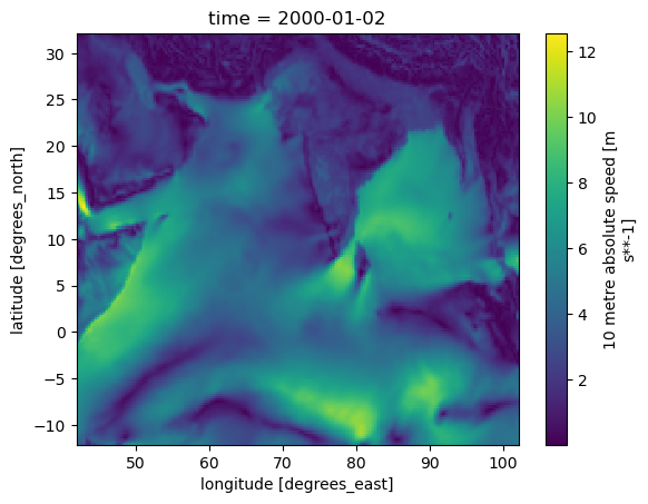
# contour map with no filling
heatmap_arr.plot.contour()
<matplotlib.contour.QuadContourSet at 0x7f7074532e90>
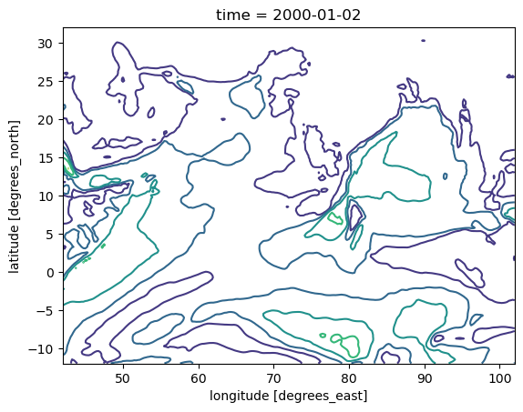
# contour map with color filling
heatmap_arr.plot.contourf()
<matplotlib.contour.QuadContourSet at 0x7f7074385890>
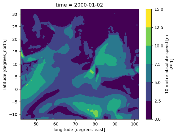
# A 3D surface plot
heatmap_arr.plot.surface()
<mpl_toolkits.mplot3d.art3d.Poly3DCollection at 0x7f7074498350>
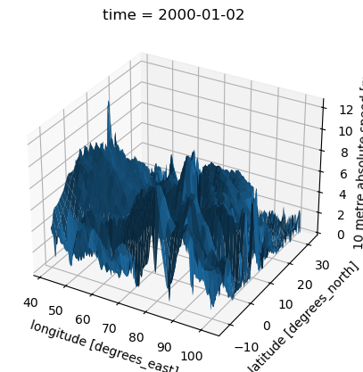
# We can create interactive plots with hvplots
heatmap_arr.hvplot().options(cmap='bgy', width=600, height=500)
Line plots#
This is mean daily wind speed by month.
ds['wind_speed'].sel(time=slice('2007', '2009')).mean(dim=['lat', 'lon']).plot(figsize=(10, 5))
[<matplotlib.lines.Line2D at 0x7f70741ea450>]

We can add in parameters to customize our graphs, as additional arguments are passed to the underlying matplotlib plot() function.
ds['air_temp'].sel(time=slice('2007', '2009')).mean(dim=['lat', 'lon']).plot.line('r-o', figsize=(10,5), markersize=1)
[<matplotlib.lines.Line2D at 0x7f70741566d0>]
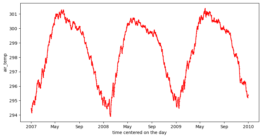
Histogram#
# creating a new Axe object if there is no currently
# available one
ax = plt.gca()
ds['wind_dir'].plot.hist(ax = ax)
ax.set_xlabel('10 metre wind direction (degrees east)')
ax.set_ylabel('frequency')
ax.set_title('Daily average wind direction distribution over covered area (1979-2022)')
Text(0.5, 1.0, 'Daily average wind direction distribution over covered area (1979-2022)')
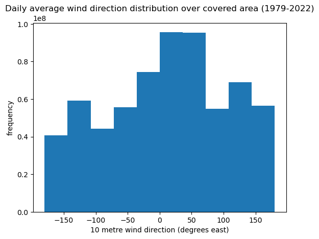
Resampling#
With xarray#
We can resample (aggregate) your data temporally. It may take a long while for the data to finish resampling, especially if your dataset is big and your resampling frequency is small.
ds_resampled = ds['CHL_cmes-gapfree'].resample(time='1ME').mean()
ds_resampled
<xarray.DataArray 'CHL_cmes-gapfree' (time: 528, lat: 177, lon: 241)> Size: 90MB
dask.array<transpose, shape=(528, 177, 241), dtype=float32, chunksize=(6, 177, 241), chunktype=numpy.ndarray>
Coordinates:
  * lat      (lat) float32 708B 32.0 31.75 31.5 31.25 ... -11.5 -11.75 -12.0
  * lon      (lon) float32 964B 42.0 42.25 42.5 42.75 ... 101.5 101.8 102.0
  * time     (time) datetime64[ns] 4kB 1979-01-31 1979-02-28 ... 2022-12-31
Attributes: (12/101)
    Conventions:                     CF-1.8, ACDD-1.3
    DPM_reference:                   GC-UD-ACRI-PUG
    IODD_reference:                  GC-UD-ACRI-PUG
    acknowledgement:                 The Licensees will ensure that original ...
    ancillary_variables:             flags CHL_uncertainty
    citation:                        The Licensees will ensure that original ...
    ...                              ...
    type:                            surface
    units:                           milligram m-3
    valid_max:                       1000.0
    valid_min:                       0.0
    westernmost_longitude:           -180.0
westernmost_valid_longitude: -180.0- time: 528
- lat: 177
- lon: 241
- dask.array<chunksize=(6, 177, 241), meta=np.ndarray>
Array Chunk Bytes 85.92 MiB 0.98 MiB Shape (528, 177, 241) (6, 177, 241) Dask graph 145 chunks in 298 graph layers Data type float32 numpy.ndarray - lat(lat)float3232.0 31.75 31.5 ... -11.75 -12.0
- long_name :
- latitude
- standard_name :
- latitude
- units :
- degrees_north
array([ 32. , 31.75, 31.5 , 31.25, 31. , 30.75, 30.5 , 30.25, 30. , 29.75, 29.5 , 29.25, 29. , 28.75, 28.5 , 28.25, 28. , 27.75, 27.5 , 27.25, 27. , 26.75, 26.5 , 26.25, 26. , 25.75, 25.5 , 25.25, 25. , 24.75, 24.5 , 24.25, 24. , 23.75, 23.5 , 23.25, 23. , 22.75, 22.5 , 22.25, 22. , 21.75, 21.5 , 21.25, 21. , 20.75, 20.5 , 20.25, 20. , 19.75, 19.5 , 19.25, 19. , 18.75, 18.5 , 18.25, 18. , 17.75, 17.5 , 17.25, 17. , 16.75, 16.5 , 16.25, 16. , 15.75, 15.5 , 15.25, 15. , 14.75, 14.5 , 14.25, 14. , 13.75, 13.5 , 13.25, 13. , 12.75, 12.5 , 12.25, 12. , 11.75, 11.5 , 11.25, 11. , 10.75, 10.5 , 10.25, 10. , 9.75, 9.5 , 9.25, 9. , 8.75, 8.5 , 8.25, 8. , 7.75, 7.5 , 7.25, 7. , 6.75, 6.5 , 6.25, 6. , 5.75, 5.5 , 5.25, 5. , 4.75, 4.5 , 4.25, 4. , 3.75, 3.5 , 3.25, 3. , 2.75, 2.5 , 2.25, 2. , 1.75, 1.5 , 1.25, 1. , 0.75, 0.5 , 0.25, 0. , -0.25, -0.5 , -0.75, -1. , -1.25, -1.5 , -1.75, -2. , -2.25, -2.5 , -2.75, -3. , -3.25, -3.5 , -3.75, -4. , -4.25, -4.5 , -4.75, -5. , -5.25, -5.5 , -5.75, -6. , -6.25, -6.5 , -6.75, -7. , -7.25, -7.5 , -7.75, -8. , -8.25, -8.5 , -8.75, -9. , -9.25, -9.5 , -9.75, -10. , -10.25, -10.5 , -10.75, -11. , -11.25, -11.5 , -11.75, -12. ], dtype=float32) - lon(lon)float3242.0 42.25 42.5 ... 101.8 102.0
- long_name :
- longitude
- standard_name :
- longitude
- units :
- degrees_east
array([ 42. , 42.25, 42.5 , ..., 101.5 , 101.75, 102. ], dtype=float32)
- time(time)datetime64[ns]1979-01-31 ... 2022-12-31
array(['1979-01-31T00:00:00.000000000', '1979-02-28T00:00:00.000000000',
       '1979-03-31T00:00:00.000000000', ..., '2022-10-31T00:00:00.000000000',
       '2022-11-30T00:00:00.000000000', '2022-12-31T00:00:00.000000000'],
      dtype='datetime64[ns]')
- latPandasIndex
PandasIndex(Index([ 32.0, 31.75, 31.5, 31.25, 31.0, 30.75, 30.5, 30.25, 30.0, 29.75, ... -9.75, -10.0, -10.25, -10.5, -10.75, -11.0, -11.25, -11.5, -11.75, -12.0], dtype='float32', name='lat', length=177)) - lonPandasIndex
PandasIndex(Index([ 42.0, 42.25, 42.5, 42.75, 43.0, 43.25, 43.5, 43.75, 44.0, 44.25, ... 99.75, 100.0, 100.25, 100.5, 100.75, 101.0, 101.25, 101.5, 101.75, 102.0], dtype='float32', name='lon', length=241)) - timePandasIndex
PandasIndex(DatetimeIndex(['1979-01-31', '1979-02-28', '1979-03-31', '1979-04-30',
               '1979-05-31', '1979-06-30', '1979-07-31', '1979-08-31',
               '1979-09-30', '1979-10-31',
               ...
               '2022-03-31', '2022-04-30', '2022-05-31', '2022-06-30',
               '2022-07-31', '2022-08-31', '2022-09-30', '2022-10-31',
               '2022-11-30', '2022-12-31'],
              dtype='datetime64[ns]', name='time', length=528, freq='ME'))
- Conventions :
- CF-1.8, ACDD-1.3
- DPM_reference :
- GC-UD-ACRI-PUG
- IODD_reference :
- GC-UD-ACRI-PUG
- acknowledgement :
- The Licensees will ensure that original CMEMS products - or value added products or derivative works developed from CMEMS Products including publications and pictures - shall credit CMEMS by explicitly making mention of the originator (CMEMS) in the following manner: <Generated using CMEMS Products, production centre ACRI-ST>
- ancillary_variables :
- flags CHL_uncertainty
- citation :
- The Licensees will ensure that original CMEMS products - or value added products or derivative works developed from CMEMS Products including publications and pictures - shall credit CMEMS by explicitly making mention of the originator (CMEMS) in the following manner: <Generated using CMEMS Products, production centre ACRI-ST>
- cmems_product_id :
- OCEANCOLOUR_GLO_BGC_L4_MY_009_104
- cmems_production_unit :
- OC-ACRI-NICE-FR
- comment :
- average
- contact :
- servicedesk.cmems@acri-st.fr
- copernicusmarine_version :
- 1.3.1
- coverage_content_type :
- modelResult
- creation_date :
- 2023-11-29 UTC
- creation_time :
- 01:06:50 UTC
- creator_email :
- servicedesk.cmems@acri-st.fr
- creator_name :
- ACRI
- creator_url :
- http://marine.copernicus.eu
- date_created :
- 2023-11-29T01:06:50Z
- distribution_statement :
- See CMEMS Data License
- duration_time :
- PT146878S
- earth_radius :
- 6378.137
- easternmost_longitude :
- 180.0
- easternmost_valid_longitude :
- 180.00001525878906
- file_quality_index :
- 0
- geospatial_bounds :
- POLYGON ((90.000000 -180.000000, 90.000000 180.000000, -90.000000 180.000000, -90.000000 -180.000000, 90.000000 -180.000000))
- geospatial_bounds_crs :
- EPSG:4326
- geospatial_bounds_vertical_crs :
- EPSG:5829
- geospatial_lat_max :
- 89.97916412353516
- geospatial_lat_min :
- -89.97917175292969
- geospatial_lon_max :
- 179.9791717529297
- geospatial_lon_min :
- -179.9791717529297
- geospatial_vertical_max :
- 0
- geospatial_vertical_min :
- 0
- geospatial_vertical_positive :
- up
- grid_mapping :
- Equirectangular
- grid_resolution :
- 4.638312339782715
- history :
- Created using software developed at ACRI-ST
- id :
- 20231121_cmems_obs-oc_glo_bgc-plankton_myint_l4-gapfree-multi-4km_P1D
- input_files_reprocessings :
- Processors versions: MODIS R2022.0NRT/VIIRSN R2022.0.1NRT/OLCIA 07.02/VIIRSJ1 R2022.0NRT/OLCIB 07.02
- institution :
- ACRI
- keywords :
- EARTH SCIENCE > OCEANS > OCEAN CHEMISTRY > CHLOROPHYLL
- keywords_vocabulary :
- NASA Global Change Master Directory (GCMD) Science Keywords
- lat_step :
- 0.0416666679084301
- license :
- See CMEMS Data License
- lon_step :
- 0.0416666679084301
- long_name :
- Chlorophyll-a concentration - Mean of the binned pixels
- naming_authority :
- CMEMS
- nb_bins :
- 37324800
- nb_equ_bins :
- 8640
- nb_grid_bins :
- 37324800
- nb_valid_bins :
- 19169208
- netcdf_version_id :
- 4.3.3.1 of Jul 8 2016 18:15:50 $
- northernmost_latitude :
- 90.0
- northernmost_valid_latitude :
- 58.08333206176758
- overall_quality :
- mode=myint
- parameter :
- Chlorophyll-a concentration
- parameter_code :
- CHL
- pct_bins :
- 100.0
- pct_valid_bins :
- 51.357831790123456
- period_duration_day :
- P1D
- period_end_day :
- 20231121
- period_start_day :
- 20231121
- platform :
- Aqua,Suomi-NPP,Sentinel-3a,JPSS-1 (NOAA-20),Sentinel-3b
- processing_level :
- L4
- product_level :
- 4
- product_name :
- 20231121_cmems_obs-oc_glo_bgc-plankton_myint_l4-gapfree-multi-4km_P1D
- product_type :
- day
- project :
- CMEMS
- publication :
- Gohin, F., Druon, J. N., Lampert, L. (2002). A five channel chlorophyll concentration algorithm applied to SeaWiFS data processed by SeaDAS in coastal waters. International journal of remote sensing, 23(8), 1639-1661 + Hu, C., Lee, Z., Franz, B. (2012). Chlorophyll a algorithms for oligotrophic oceans: A novel approach based on three-band reflectance difference. Journal of Geophysical Research, 117(C1). doi: 10.1029/2011jc007395
- publisher_email :
- servicedesk.cmems@mercator-ocean.eu
- publisher_name :
- CMEMS
- publisher_url :
- http://marine.copernicus.eu
- references :
- http://www.globcolour.info GlobColour has been originally funded by ESA with data from ESA, NASA, NOAA and GeoEye. This version has received funding from the European Community s Seventh Framework Programme ([FP7/2007-2013]) under grant agreement n. 282723 [OSS2015 project].
- registration :
- 5
- sensor :
- Moderate Resolution Imaging Spectroradiometer,Visible Infrared Imaging Radiometer Suite,Ocean and Land Colour Instrument
- sensor_name :
- MODISA,VIIRSN,OLCIa,VIIRSJ1,OLCIb
- sensor_name_list :
- MOD,VIR,OLA,VJ1,OLB
- site_name :
- GLO
- software_name :
- globcolour_l3_reproject
- software_version :
- 2022.2
- source :
- surface observation
- southernmost_latitude :
- -90.0
- southernmost_valid_latitude :
- -78.58333587646484
- standard_name :
- mass_concentration_of_chlorophyll_a_in_sea_water
- standard_name_vocabulary :
- NetCDF Climate and Forecast (CF) Metadata Convention
- start_date :
- 2023-11-20 UTC
- start_time :
- 15:24:55 UTC
- stop_date :
- 2023-11-22 UTC
- stop_time :
- 08:12:52 UTC
- summary :
- CMEMS product: cmems_obs-oc_glo_bgc-plankton_my_l4-gapfree-multi-4km_P1D, generated by ACRI-ST
- time_coverage_duration :
- PT146878S
- time_coverage_end :
- 2023-11-22T08:12:52Z
- time_coverage_resolution :
- P1D
- time_coverage_start :
- 2023-11-20T15:24:55Z
- title :
- cmems_obs-oc_glo_bgc-plankton_my_l4-gapfree-multi-4km_P1D
- type :
- surface
- units :
- milligram m-3
- valid_max :
- 1000.0
- valid_min :
- 0.0
- westernmost_longitude :
- -180.0
- westernmost_valid_longitude :
- -180.0
We can see that after resampling, our time dimension size is reduced from days to months.
CHL_month = ds_resampled.mean(dim=['lat', 'lon']).hvplot(label='monthly resampling').options(color='red', )
CHL_month
CHL_day = ds['CHL_cmes-gapfree'].mean(dim=['lat', 'lon']).hvplot(label='daily resampling').options(color='blue')
CHL_day
(CHL_day*CHL_month).options(title='Monthly vs Daily resampling of chlorophyll-a levels', xlabel='year')