Preparing a Zarr dataset for our CNN training#
Author: Eli Holmes (NOAA)
Goal an xarray Dataset#
For fitting our CNN model with TensorFlow, we want an xarray Dataset with our predictors and response variables. We need the variables to be chunked dask arrays. The time dimension should be named time and grid lat and lon, for use in my fitting code. We also need an ocean mask.
Summary of the steps#
Subset to a smaller spatial region
Subset to only the variables I need
Get rid of days with many NaNs
Save in Zarr format. Why Zarr? It is a standard ML-optimized format for gridded data.
Chunked & lazy loading: Keeps your Dask chunking intact.
Efficient: Only loads the data you need into memory.
Parallel IO: Works great with Dask for scalable access.
Flexible: Plays well with training pipelines in TensorFlow or PyTorch via prefetching or conversion.
Load the libraries that we need#
# --- Core data handling libraries ---
import xarray as xr       # for working with labeled multi-dimensional arrays
import numpy as np        # for numerical operations on arrays
import dask.array as da   # for lazy, parallel array operations (used in xarray backends)

# --- Plotting ---
import matplotlib.pyplot as plt  # for creating plots
Load data#
For Part I, we will use a data set in the shared drive. In Part II, we will look at streaming data from the cloud.
# read in the Zarr file; a 3D (time, lat, lon) cube for a bunch of variables in the Indian Ocean
zarr_ds = xr.open_zarr("~/shared/mind_the_chl_gap/IO.zarr")
zarr_ds
<xarray.Dataset> Size: 66GB
Dimensions:                       (time: 16071, lat: 177, lon: 241)
Coordinates:
  * lat                           (lat) float32 708B 32.0 31.75 ... -11.75 -12.0
  * lon                           (lon) float32 964B 42.0 42.25 ... 101.8 102.0
  * time                          (time) datetime64[ns] 129kB 1979-01-01 ... ...
Data variables: (12/27)
    CHL                           (time, lat, lon) float32 3GB dask.array<chunksize=(100, 177, 241), meta=np.ndarray>
    CHL_cmes-cloud                (time, lat, lon) uint8 686MB dask.array<chunksize=(100, 177, 241), meta=np.ndarray>
    CHL_cmes-gapfree              (time, lat, lon) float32 3GB dask.array<chunksize=(100, 177, 241), meta=np.ndarray>
    CHL_cmes-land                 (lat, lon) uint8 43kB dask.array<chunksize=(177, 241), meta=np.ndarray>
    CHL_cmes-level3               (time, lat, lon) float32 3GB dask.array<chunksize=(100, 177, 241), meta=np.ndarray>
    CHL_cmes_flags-gapfree        (time, lat, lon) float32 3GB dask.array<chunksize=(100, 177, 241), meta=np.ndarray>
    ...                            ...
    ug_curr                       (time, lat, lon) float32 3GB dask.array<chunksize=(100, 177, 241), meta=np.ndarray>
    v_curr                        (time, lat, lon) float32 3GB dask.array<chunksize=(100, 177, 241), meta=np.ndarray>
    v_wind                        (time, lat, lon) float32 3GB dask.array<chunksize=(100, 177, 241), meta=np.ndarray>
    vg_curr                       (time, lat, lon) float32 3GB dask.array<chunksize=(100, 177, 241), meta=np.ndarray>
    wind_dir                      (time, lat, lon) float32 3GB dask.array<chunksize=(100, 177, 241), meta=np.ndarray>
    wind_speed                    (time, lat, lon) float32 3GB dask.array<chunksize=(100, 177, 241), meta=np.ndarray>
Attributes: (12/92)
    Conventions:                     CF-1.8, ACDD-1.3
    DPM_reference:                   GC-UD-ACRI-PUG
    IODD_reference:                  GC-UD-ACRI-PUG
    acknowledgement:                 The Licensees will ensure that original ...
    citation:                        The Licensees will ensure that original ...
    cmems_product_id:                OCEANCOLOUR_GLO_BGC_L3_MY_009_103
    ...                              ...
    time_coverage_end:               2024-04-18T02:58:23Z
    time_coverage_resolution:        P1D
    time_coverage_start:             2024-04-16T21:12:05Z
    title:                           cmems_obs-oc_glo_bgc-plankton_my_l3-mult...
    westernmost_longitude:           -180.0
westernmost_valid_longitude: -180.0- time: 16071
- lat: 177
- lon: 241
- lat(lat)float3232.0 31.75 31.5 ... -11.75 -12.0
- long_name :
- latitude
- standard_name :
- latitude
- units :
- degrees_north
array([ 32. , 31.75, 31.5 , 31.25, 31. , 30.75, 30.5 , 30.25, 30. , 29.75, 29.5 , 29.25, 29. , 28.75, 28.5 , 28.25, 28. , 27.75, 27.5 , 27.25, 27. , 26.75, 26.5 , 26.25, 26. , 25.75, 25.5 , 25.25, 25. , 24.75, 24.5 , 24.25, 24. , 23.75, 23.5 , 23.25, 23. , 22.75, 22.5 , 22.25, 22. , 21.75, 21.5 , 21.25, 21. , 20.75, 20.5 , 20.25, 20. , 19.75, 19.5 , 19.25, 19. , 18.75, 18.5 , 18.25, 18. , 17.75, 17.5 , 17.25, 17. , 16.75, 16.5 , 16.25, 16. , 15.75, 15.5 , 15.25, 15. , 14.75, 14.5 , 14.25, 14. , 13.75, 13.5 , 13.25, 13. , 12.75, 12.5 , 12.25, 12. , 11.75, 11.5 , 11.25, 11. , 10.75, 10.5 , 10.25, 10. , 9.75, 9.5 , 9.25, 9. , 8.75, 8.5 , 8.25, 8. , 7.75, 7.5 , 7.25, 7. , 6.75, 6.5 , 6.25, 6. , 5.75, 5.5 , 5.25, 5. , 4.75, 4.5 , 4.25, 4. , 3.75, 3.5 , 3.25, 3. , 2.75, 2.5 , 2.25, 2. , 1.75, 1.5 , 1.25, 1. , 0.75, 0.5 , 0.25, 0. , -0.25, -0.5 , -0.75, -1. , -1.25, -1.5 , -1.75, -2. , -2.25, -2.5 , -2.75, -3. , -3.25, -3.5 , -3.75, -4. , -4.25, -4.5 , -4.75, -5. , -5.25, -5.5 , -5.75, -6. , -6.25, -6.5 , -6.75, -7. , -7.25, -7.5 , -7.75, -8. , -8.25, -8.5 , -8.75, -9. , -9.25, -9.5 , -9.75, -10. , -10.25, -10.5 , -10.75, -11. , -11.25, -11.5 , -11.75, -12. ], dtype=float32) - lon(lon)float3242.0 42.25 42.5 ... 101.8 102.0
- long_name :
- longitude
- standard_name :
- longitude
- units :
- degrees_east
array([ 42. , 42.25, 42.5 , ..., 101.5 , 101.75, 102. ], dtype=float32)
- time(time)datetime64[ns]1979-01-01 ... 2022-12-31
- axis :
- T
- comment :
- Data is averaged over the day
- long_name :
- time centered on the day
- standard_name :
- time
- time_bounds :
- 2000-01-01 00:00:00 to 2000-01-01 23:59:59
array(['1979-01-01T00:00:00.000000000', '1979-01-02T00:00:00.000000000',
       '1979-01-03T00:00:00.000000000', ..., '2022-12-29T00:00:00.000000000',
       '2022-12-30T00:00:00.000000000', '2022-12-31T00:00:00.000000000'],
      dtype='datetime64[ns]')
- CHL(time, lat, lon)float32dask.array<chunksize=(100, 177, 241), meta=np.ndarray>
- _ChunkSizes :
- [1, 256, 256]
- ancillary_variables :
- flags CHL_uncertainty
- coverage_content_type :
- modelResult
- input_files_reprocessings :
- Processors versions: MODIS R2022.0NRT/VIIRSN R2022.0NRT/OLCIA 07.02/VIIRSJ1 R2022.0NRT/OLCIB 07.02
- long_name :
- Chlorophyll-a concentration - Mean of the binned pixels
- standard_name :
- mass_concentration_of_chlorophyll_a_in_sea_water
- type :
- surface
- units :
- milligram m-3
- valid_max :
- 1000.0
- valid_min :
- 0.0
Array Chunk Bytes 2.55 GiB 16.27 MiB Shape (16071, 177, 241) (100, 177, 241) Dask graph 161 chunks in 2 graph layers Data type float32 numpy.ndarray - CHL_cmes-cloud(time, lat, lon)uint8dask.array<chunksize=(100, 177, 241), meta=np.ndarray>
- title :
- flag for CHL-gapfree and CHL-level3. 0 is land; 1 is cloud; 0 is water
Array Chunk Bytes 653.78 MiB 4.07 MiB Shape (16071, 177, 241) (100, 177, 241) Dask graph 161 chunks in 2 graph layers Data type uint8 numpy.ndarray - CHL_cmes-gapfree(time, lat, lon)float32dask.array<chunksize=(100, 177, 241), meta=np.ndarray>
- Conventions :
- CF-1.8, ACDD-1.3
- DPM_reference :
- GC-UD-ACRI-PUG
- IODD_reference :
- GC-UD-ACRI-PUG
- acknowledgement :
- The Licensees will ensure that original CMEMS products - or value added products or derivative works developed from CMEMS Products including publications and pictures - shall credit CMEMS by explicitly making mention of the originator (CMEMS) in the following manner: <Generated using CMEMS Products, production centre ACRI-ST>
- ancillary_variables :
- flags CHL_uncertainty
- citation :
- The Licensees will ensure that original CMEMS products - or value added products or derivative works developed from CMEMS Products including publications and pictures - shall credit CMEMS by explicitly making mention of the originator (CMEMS) in the following manner: <Generated using CMEMS Products, production centre ACRI-ST>
- cmems_product_id :
- OCEANCOLOUR_GLO_BGC_L4_MY_009_104
- cmems_production_unit :
- OC-ACRI-NICE-FR
- comment :
- average
- contact :
- servicedesk.cmems@acri-st.fr
- copernicusmarine_version :
- 1.3.1
- coverage_content_type :
- modelResult
- creation_date :
- 2023-11-29 UTC
- creation_time :
- 01:06:50 UTC
- creator_email :
- servicedesk.cmems@acri-st.fr
- creator_name :
- ACRI
- creator_url :
- http://marine.copernicus.eu
- date_created :
- 2023-11-29T01:06:50Z
- distribution_statement :
- See CMEMS Data License
- duration_time :
- PT146878S
- earth_radius :
- 6378.137
- easternmost_longitude :
- 180.0
- easternmost_valid_longitude :
- 180.00001525878906
- file_quality_index :
- 0
- geospatial_bounds :
- POLYGON ((90.000000 -180.000000, 90.000000 180.000000, -90.000000 180.000000, -90.000000 -180.000000, 90.000000 -180.000000))
- geospatial_bounds_crs :
- EPSG:4326
- geospatial_bounds_vertical_crs :
- EPSG:5829
- geospatial_lat_max :
- 89.97916412353516
- geospatial_lat_min :
- -89.97917175292969
- geospatial_lon_max :
- 179.9791717529297
- geospatial_lon_min :
- -179.9791717529297
- geospatial_vertical_max :
- 0
- geospatial_vertical_min :
- 0
- geospatial_vertical_positive :
- up
- grid_mapping :
- Equirectangular
- grid_resolution :
- 4.638312339782715
- history :
- Created using software developed at ACRI-ST
- id :
- 20231121_cmems_obs-oc_glo_bgc-plankton_myint_l4-gapfree-multi-4km_P1D
- input_files_reprocessings :
- Processors versions: MODIS R2022.0NRT/VIIRSN R2022.0.1NRT/OLCIA 07.02/VIIRSJ1 R2022.0NRT/OLCIB 07.02
- institution :
- ACRI
- keywords :
- EARTH SCIENCE > OCEANS > OCEAN CHEMISTRY > CHLOROPHYLL
- keywords_vocabulary :
- NASA Global Change Master Directory (GCMD) Science Keywords
- lat_step :
- 0.0416666679084301
- license :
- See CMEMS Data License
- lon_step :
- 0.0416666679084301
- long_name :
- Chlorophyll-a concentration - Mean of the binned pixels
- naming_authority :
- CMEMS
- nb_bins :
- 37324800
- nb_equ_bins :
- 8640
- nb_grid_bins :
- 37324800
- nb_valid_bins :
- 19169208
- netcdf_version_id :
- 4.3.3.1 of Jul 8 2016 18:15:50 $
- northernmost_latitude :
- 90.0
- northernmost_valid_latitude :
- 58.08333206176758
- overall_quality :
- mode=myint
- parameter :
- Chlorophyll-a concentration
- parameter_code :
- CHL
- pct_bins :
- 100.0
- pct_valid_bins :
- 51.357831790123456
- period_duration_day :
- P1D
- period_end_day :
- 20231121
- period_start_day :
- 20231121
- platform :
- Aqua,Suomi-NPP,Sentinel-3a,JPSS-1 (NOAA-20),Sentinel-3b
- processing_level :
- L4
- product_level :
- 4
- product_name :
- 20231121_cmems_obs-oc_glo_bgc-plankton_myint_l4-gapfree-multi-4km_P1D
- product_type :
- day
- project :
- CMEMS
- publication :
- Gohin, F., Druon, J. N., Lampert, L. (2002). A five channel chlorophyll concentration algorithm applied to SeaWiFS data processed by SeaDAS in coastal waters. International journal of remote sensing, 23(8), 1639-1661 + Hu, C., Lee, Z., Franz, B. (2012). Chlorophyll a algorithms for oligotrophic oceans: A novel approach based on three-band reflectance difference. Journal of Geophysical Research, 117(C1). doi: 10.1029/2011jc007395
- publisher_email :
- servicedesk.cmems@mercator-ocean.eu
- publisher_name :
- CMEMS
- publisher_url :
- http://marine.copernicus.eu
- references :
- http://www.globcolour.info GlobColour has been originally funded by ESA with data from ESA, NASA, NOAA and GeoEye. This version has received funding from the European Community s Seventh Framework Programme ([FP7/2007-2013]) under grant agreement n. 282723 [OSS2015 project].
- registration :
- 5
- sensor :
- Moderate Resolution Imaging Spectroradiometer,Visible Infrared Imaging Radiometer Suite,Ocean and Land Colour Instrument
- sensor_name :
- MODISA,VIIRSN,OLCIa,VIIRSJ1,OLCIb
- sensor_name_list :
- MOD,VIR,OLA,VJ1,OLB
- site_name :
- GLO
- software_name :
- globcolour_l3_reproject
- software_version :
- 2022.2
- source :
- surface observation
- southernmost_latitude :
- -90.0
- southernmost_valid_latitude :
- -78.58333587646484
- standard_name :
- mass_concentration_of_chlorophyll_a_in_sea_water
- standard_name_vocabulary :
- NetCDF Climate and Forecast (CF) Metadata Convention
- start_date :
- 2023-11-20 UTC
- start_time :
- 15:24:55 UTC
- stop_date :
- 2023-11-22 UTC
- stop_time :
- 08:12:52 UTC
- summary :
- CMEMS product: cmems_obs-oc_glo_bgc-plankton_my_l4-gapfree-multi-4km_P1D, generated by ACRI-ST
- time_coverage_duration :
- PT146878S
- time_coverage_end :
- 2023-11-22T08:12:52Z
- time_coverage_resolution :
- P1D
- time_coverage_start :
- 2023-11-20T15:24:55Z
- title :
- cmems_obs-oc_glo_bgc-plankton_my_l4-gapfree-multi-4km_P1D
- type :
- surface
- units :
- milligram m-3
- valid_max :
- 1000.0
- valid_min :
- 0.0
- westernmost_longitude :
- -180.0
- westernmost_valid_longitude :
- -180.0
Array Chunk Bytes 2.55 GiB 16.27 MiB Shape (16071, 177, 241) (100, 177, 241) Dask graph 161 chunks in 2 graph layers Data type float32 numpy.ndarray - CHL_cmes-land(lat, lon)uint8dask.array<chunksize=(177, 241), meta=np.ndarray>
Array Chunk Bytes 41.66 kiB 41.66 kiB Shape (177, 241) (177, 241) Dask graph 1 chunks in 2 graph layers Data type uint8 numpy.ndarray - CHL_cmes-level3(time, lat, lon)float32dask.array<chunksize=(100, 177, 241), meta=np.ndarray>
- Conventions :
- CF-1.8, ACDD-1.3
- DPM_reference :
- GC-UD-ACRI-PUG
- IODD_reference :
- GC-UD-ACRI-PUG
- acknowledgement :
- The Licensees will ensure that original CMEMS products - or value added products or derivative works developed from CMEMS Products including publications and pictures - shall credit CMEMS by explicitly making mention of the originator (CMEMS) in the following manner: <Generated using CMEMS Products, production centre ACRI-ST>
- ancillary_variables :
- flags CHL_uncertainty
- citation :
- The Licensees will ensure that original CMEMS products - or value added products or derivative works developed from CMEMS Products including publications and pictures - shall credit CMEMS by explicitly making mention of the originator (CMEMS) in the following manner: <Generated using CMEMS Products, production centre ACRI-ST>
- cmems_product_id :
- OCEANCOLOUR_GLO_BGC_L3_MY_009_103
- cmems_production_unit :
- OC-ACRI-NICE-FR
- comment :
- average
- contact :
- servicedesk.cmems@acri-st.fr
- copernicusmarine_version :
- 1.3.1
- coverage_content_type :
- modelResult
- creation_date :
- 2024-04-25 UTC
- creation_time :
- 00:47:33 UTC
- creator_email :
- servicedesk.cmems@acri-st.fr
- creator_name :
- ACRI
- creator_url :
- http://marine.copernicus.eu
- date_created :
- 2024-04-25T00:47:33Z
- distribution_statement :
- See CMEMS Data License
- duration_time :
- PT107179S
- earth_radius :
- 6378.137
- easternmost_longitude :
- 180.0
- easternmost_valid_longitude :
- 180.00001525878906
- file_quality_index :
- 0
- geospatial_bounds :
- POLYGON ((90.000000 -180.000000, 90.000000 180.000000, -90.000000 180.000000, -90.000000 -180.000000, 90.000000 -180.000000))
- geospatial_bounds_crs :
- EPSG:4326
- geospatial_bounds_vertical_crs :
- EPSG:5829
- geospatial_lat_max :
- 89.97916412353516
- geospatial_lat_min :
- -89.97917175292969
- geospatial_lon_max :
- 179.9791717529297
- geospatial_lon_min :
- -179.9791717529297
- geospatial_vertical_max :
- 0
- geospatial_vertical_min :
- 0
- geospatial_vertical_positive :
- up
- grid_mapping :
- Equirectangular
- grid_resolution :
- 4.638312339782715
- history :
- Created using software developed at ACRI-ST
- id :
- 20240417_cmems_obs-oc_glo_bgc-plankton_myint_l3-multi-4km_P1D
- input_files_reprocessings :
- Processors versions: MODIS R2022.0NRT/VIIRSN R2022.0.1NRT/OLCIA 07.04/VIIRSJ1 R2022.0NRT/OLCIB 07.04
- institution :
- ACRI
- keywords :
- EARTH SCIENCE > OCEANS > OCEAN CHEMISTRY > CHLOROPHYLL, EARTH SCIENCE > BIOLOGICAL CLASSIFICATION > PROTISTS > PLANKTON > PHYTOPLANKTON
- keywords_vocabulary :
- NASA Global Change Master Directory (GCMD) Science Keywords
- lat_step :
- 0.0416666679084301
- license :
- See CMEMS Data License
- lon_step :
- 0.0416666679084301
- long_name :
- Chlorophyll-a concentration - Mean of the binned pixels
- naming_authority :
- CMEMS
- nb_bins :
- 37324800
- nb_equ_bins :
- 8640
- nb_grid_bins :
- 37324800
- nb_valid_bins :
- 9704694
- netcdf_version_id :
- 4.3.3.1 of Jul 8 2016 18:15:50 $
- northernmost_latitude :
- 90.0
- northernmost_valid_latitude :
- 82.70833587646484
- overall_quality :
- mode=myint
- parameter :
- Chlorophyll-a concentration,Phytoplankton Functional Types
- parameter_code :
- CHL,DIATO,DINO,HAPTO,GREEN,PROKAR,PROCHLO,MICRO,NANO,PICO
- pct_bins :
- 100.0
- pct_valid_bins :
- 26.000659079218106
- period_duration_day :
- P1D
- period_end_day :
- 20240417
- period_start_day :
- 20240417
- platform :
- Aqua,Suomi-NPP,Sentinel-3a,JPSS-1 (NOAA-20),Sentinel-3b
- processing_level :
- L3
- product_level :
- 3
- product_name :
- 20240417_cmems_obs-oc_glo_bgc-plankton_myint_l3-multi-4km_P1D
- product_type :
- day
- project :
- CMEMS
- publication :
- Gohin, F., Druon, J. N., Lampert, L. (2002). A five channel chlorophyll concentration algorithm applied to SeaWiFS data processed by SeaDAS in coastal waters. International journal of remote sensing, 23(8), 1639-1661 + Hu, C., Lee, Z., Franz, B. (2012). Chlorophyll a algorithms for oligotrophic oceans: A novel approach based on three-band reflectance difference. Journal of Geophysical Research, 117(C1). doi: 10.1029/2011jc007395 + Xi H, Losa S N, Mangin A, Garnesson P, Bretagnon M, Demaria J, Soppa M A, Hembise Fanton d Andon O, Bracher A (2021) Global chlorophyll a concentrations of phytoplankton functional types with detailed uncertainty assessment using multi-sensor ocean color and sea surface temperature satellite products, JGR, in review.
- publisher_email :
- servicedesk.cmems@mercator-ocean.eu
- publisher_name :
- CMEMS
- publisher_url :
- http://marine.copernicus.eu
- references :
- http://www.globcolour.info GlobColour has been originally funded by ESA with data from ESA, NASA, NOAA and GeoEye. This version has received funding from the European Community s Seventh Framework Programme ([FP7/2007-2013]) under grant agreement n. 282723 [OSS2015 project].
- registration :
- 5
- sensor :
- Moderate Resolution Imaging Spectroradiometer,Visible Infrared Imaging Radiometer Suite,Ocean and Land Colour Instrument
- sensor_name :
- MODISA,VIIRSN,OLCIa,VIIRSJ1,OLCIb
- sensor_name_list :
- MOD,VIR,OLA,VJ1,OLB
- site_name :
- GLO
- software_name :
- globcolour_l3_reproject
- software_version :
- 2022.2
- source :
- surface observation
- southernmost_latitude :
- -90.0
- southernmost_valid_latitude :
- -66.33333587646484
- standard_name :
- mass_concentration_of_chlorophyll_a_in_sea_water
- standard_name_vocabulary :
- NetCDF Climate and Forecast (CF) Metadata Convention
- start_date :
- 2024-04-16 UTC
- start_time :
- 21:12:05 UTC
- stop_date :
- 2024-04-18 UTC
- stop_time :
- 02:58:23 UTC
- summary :
- CMEMS product: cmems_obs-oc_glo_bgc-plankton_my_l3-multi-4km_P1D, generated by ACRI-ST
- time_coverage_duration :
- PT107179S
- time_coverage_end :
- 2024-04-18T02:58:23Z
- time_coverage_resolution :
- P1D
- time_coverage_start :
- 2024-04-16T21:12:05Z
- title :
- cmems_obs-oc_glo_bgc-plankton_my_l3-multi-4km_P1D
- type :
- surface
- units :
- milligram m-3
- valid_max :
- 1000.0
- valid_min :
- 0.0
- westernmost_longitude :
- -180.0
- westernmost_valid_longitude :
- -180.0
Array Chunk Bytes 2.55 GiB 16.27 MiB Shape (16071, 177, 241) (100, 177, 241) Dask graph 161 chunks in 2 graph layers Data type float32 numpy.ndarray - CHL_cmes_flags-gapfree(time, lat, lon)float32dask.array<chunksize=(100, 177, 241), meta=np.ndarray>
- Conventions :
- CF-1.8, ACDD-1.3
- DPM_reference :
- GC-UD-ACRI-PUG
- IODD_reference :
- GC-UD-ACRI-PUG
- acknowledgement :
- The Licensees will ensure that original CMEMS products - or value added products or derivative works developed from CMEMS Products including publications and pictures - shall credit CMEMS by explicitly making mention of the originator (CMEMS) in the following manner: <Generated using CMEMS Products, production centre ACRI-ST>
- citation :
- The Licensees will ensure that original CMEMS products - or value added products or derivative works developed from CMEMS Products including publications and pictures - shall credit CMEMS by explicitly making mention of the originator (CMEMS) in the following manner: <Generated using CMEMS Products, production centre ACRI-ST>
- cmems_product_id :
- OCEANCOLOUR_GLO_BGC_L4_MY_009_104
- cmems_production_unit :
- OC-ACRI-NICE-FR
- comment :
- average
- contact :
- servicedesk.cmems@acri-st.fr
- copernicusmarine_version :
- 1.3.1
- coverage_content_type :
- auxiliaryInformation
- creation_date :
- 2023-11-29 UTC
- creation_time :
- 01:06:50 UTC
- creator_email :
- servicedesk.cmems@acri-st.fr
- creator_name :
- ACRI
- creator_url :
- http://marine.copernicus.eu
- date_created :
- 2023-11-29T01:06:50Z
- distribution_statement :
- See CMEMS Data License
- duration_time :
- PT146878S
- earth_radius :
- 6378.137
- easternmost_longitude :
- 180.0
- easternmost_valid_longitude :
- 180.00001525878906
- file_quality_index :
- 0
- flag_masks :
- [1, 2]
- flag_meanings :
- LAND INTERPOLATED
- geospatial_bounds :
- POLYGON ((90.000000 -180.000000, 90.000000 180.000000, -90.000000 180.000000, -90.000000 -180.000000, 90.000000 -180.000000))
- geospatial_bounds_crs :
- EPSG:4326
- geospatial_bounds_vertical_crs :
- EPSG:5829
- geospatial_lat_max :
- 89.97916412353516
- geospatial_lat_min :
- -89.97917175292969
- geospatial_lon_max :
- 179.9791717529297
- geospatial_lon_min :
- -179.9791717529297
- geospatial_vertical_max :
- 0
- geospatial_vertical_min :
- 0
- geospatial_vertical_positive :
- up
- grid_mapping :
- Equirectangular
- grid_resolution :
- 4.638312339782715
- history :
- Created using software developed at ACRI-ST
- id :
- 20231121_cmems_obs-oc_glo_bgc-plankton_myint_l4-gapfree-multi-4km_P1D
- institution :
- ACRI
- keywords :
- EARTH SCIENCE > OCEANS > OCEAN CHEMISTRY > CHLOROPHYLL
- keywords_vocabulary :
- NASA Global Change Master Directory (GCMD) Science Keywords
- lat_step :
- 0.0416666679084301
- license :
- See CMEMS Data License
- lon_step :
- 0.0416666679084301
- long_name :
- Flags
- naming_authority :
- CMEMS
- nb_bins :
- 37324800
- nb_equ_bins :
- 8640
- nb_grid_bins :
- 37324800
- nb_valid_bins :
- 19169208
- netcdf_version_id :
- 4.3.3.1 of Jul 8 2016 18:15:50 $
- northernmost_latitude :
- 90.0
- northernmost_valid_latitude :
- 58.08333206176758
- overall_quality :
- mode=myint
- parameter :
- Chlorophyll-a concentration
- parameter_code :
- CHL
- pct_bins :
- 100.0
- pct_valid_bins :
- 51.357831790123456
- period_duration_day :
- P1D
- period_end_day :
- 20231121
- period_start_day :
- 20231121
- platform :
- Aqua,Suomi-NPP,Sentinel-3a,JPSS-1 (NOAA-20),Sentinel-3b
- processing_level :
- L4
- product_level :
- 4
- product_name :
- 20231121_cmems_obs-oc_glo_bgc-plankton_myint_l4-gapfree-multi-4km_P1D
- product_type :
- day
- project :
- CMEMS
- publication :
- Gohin, F., Druon, J. N., Lampert, L. (2002). A five channel chlorophyll concentration algorithm applied to SeaWiFS data processed by SeaDAS in coastal waters. International journal of remote sensing, 23(8), 1639-1661 + Hu, C., Lee, Z., Franz, B. (2012). Chlorophyll a algorithms for oligotrophic oceans: A novel approach based on three-band reflectance difference. Journal of Geophysical Research, 117(C1). doi: 10.1029/2011jc007395
- publisher_email :
- servicedesk.cmems@mercator-ocean.eu
- publisher_name :
- CMEMS
- publisher_url :
- http://marine.copernicus.eu
- references :
- http://www.globcolour.info GlobColour has been originally funded by ESA with data from ESA, NASA, NOAA and GeoEye. This version has received funding from the European Community s Seventh Framework Programme ([FP7/2007-2013]) under grant agreement n. 282723 [OSS2015 project].
- registration :
- 5
- sensor :
- Moderate Resolution Imaging Spectroradiometer,Visible Infrared Imaging Radiometer Suite,Ocean and Land Colour Instrument
- sensor_name :
- MODISA,VIIRSN,OLCIa,VIIRSJ1,OLCIb
- sensor_name_list :
- MOD,VIR,OLA,VJ1,OLB
- site_name :
- GLO
- software_name :
- globcolour_l3_reproject
- software_version :
- 2022.2
- source :
- surface observation
- southernmost_latitude :
- -90.0
- southernmost_valid_latitude :
- -78.58333587646484
- standard_name :
- status_flag
- standard_name_vocabulary :
- NetCDF Climate and Forecast (CF) Metadata Convention
- start_date :
- 2023-11-20 UTC
- start_time :
- 15:24:55 UTC
- stop_date :
- 2023-11-22 UTC
- stop_time :
- 08:12:52 UTC
- summary :
- CMEMS product: cmems_obs-oc_glo_bgc-plankton_my_l4-gapfree-multi-4km_P1D, generated by ACRI-ST
- time_coverage_duration :
- PT146878S
- time_coverage_end :
- 2023-11-22T08:12:52Z
- time_coverage_resolution :
- P1D
- time_coverage_start :
- 2023-11-20T15:24:55Z
- title :
- cmems_obs-oc_glo_bgc-plankton_my_l4-gapfree-multi-4km_P1D
- valid_max :
- 3
- valid_min :
- 0
- westernmost_longitude :
- -180.0
- westernmost_valid_longitude :
- -180.0
Array Chunk Bytes 2.55 GiB 16.27 MiB Shape (16071, 177, 241) (100, 177, 241) Dask graph 161 chunks in 2 graph layers Data type float32 numpy.ndarray - CHL_cmes_flags-level3(time, lat, lon)float32dask.array<chunksize=(100, 177, 241), meta=np.ndarray>
- Conventions :
- CF-1.8, ACDD-1.3
- DPM_reference :
- GC-UD-ACRI-PUG
- IODD_reference :
- GC-UD-ACRI-PUG
- acknowledgement :
- The Licensees will ensure that original CMEMS products - or value added products or derivative works developed from CMEMS Products including publications and pictures - shall credit CMEMS by explicitly making mention of the originator (CMEMS) in the following manner: <Generated using CMEMS Products, production centre ACRI-ST>
- citation :
- The Licensees will ensure that original CMEMS products - or value added products or derivative works developed from CMEMS Products including publications and pictures - shall credit CMEMS by explicitly making mention of the originator (CMEMS) in the following manner: <Generated using CMEMS Products, production centre ACRI-ST>
- cmems_product_id :
- OCEANCOLOUR_GLO_BGC_L3_MY_009_103
- cmems_production_unit :
- OC-ACRI-NICE-FR
- comment :
- average
- contact :
- servicedesk.cmems@acri-st.fr
- copernicusmarine_version :
- 1.3.1
- coverage_content_type :
- auxiliaryInformation
- creation_date :
- 2024-04-25 UTC
- creation_time :
- 00:47:33 UTC
- creator_email :
- servicedesk.cmems@acri-st.fr
- creator_name :
- ACRI
- creator_url :
- http://marine.copernicus.eu
- date_created :
- 2024-04-25T00:47:33Z
- distribution_statement :
- See CMEMS Data License
- duration_time :
- PT107179S
- earth_radius :
- 6378.137
- easternmost_longitude :
- 180.0
- easternmost_valid_longitude :
- 180.00001525878906
- file_quality_index :
- 0
- flag_masks :
- 1
- flag_meanings :
- LAND
- geospatial_bounds :
- POLYGON ((90.000000 -180.000000, 90.000000 180.000000, -90.000000 180.000000, -90.000000 -180.000000, 90.000000 -180.000000))
- geospatial_bounds_crs :
- EPSG:4326
- geospatial_bounds_vertical_crs :
- EPSG:5829
- geospatial_lat_max :
- 89.97916412353516
- geospatial_lat_min :
- -89.97917175292969
- geospatial_lon_max :
- 179.9791717529297
- geospatial_lon_min :
- -179.9791717529297
- geospatial_vertical_max :
- 0
- geospatial_vertical_min :
- 0
- geospatial_vertical_positive :
- up
- grid_mapping :
- Equirectangular
- grid_resolution :
- 4.638312339782715
- history :
- Created using software developed at ACRI-ST
- id :
- 20240417_cmems_obs-oc_glo_bgc-plankton_myint_l3-multi-4km_P1D
- institution :
- ACRI
- keywords :
- EARTH SCIENCE > OCEANS > OCEAN CHEMISTRY > CHLOROPHYLL, EARTH SCIENCE > BIOLOGICAL CLASSIFICATION > PROTISTS > PLANKTON > PHYTOPLANKTON
- keywords_vocabulary :
- NASA Global Change Master Directory (GCMD) Science Keywords
- lat_step :
- 0.0416666679084301
- license :
- See CMEMS Data License
- lon_step :
- 0.0416666679084301
- long_name :
- Flags
- naming_authority :
- CMEMS
- nb_bins :
- 37324800
- nb_equ_bins :
- 8640
- nb_grid_bins :
- 37324800
- nb_valid_bins :
- 9704694
- netcdf_version_id :
- 4.3.3.1 of Jul 8 2016 18:15:50 $
- northernmost_latitude :
- 90.0
- northernmost_valid_latitude :
- 82.70833587646484
- overall_quality :
- mode=myint
- parameter :
- Chlorophyll-a concentration,Phytoplankton Functional Types
- parameter_code :
- CHL,DIATO,DINO,HAPTO,GREEN,PROKAR,PROCHLO,MICRO,NANO,PICO
- pct_bins :
- 100.0
- pct_valid_bins :
- 26.000659079218106
- period_duration_day :
- P1D
- period_end_day :
- 20240417
- period_start_day :
- 20240417
- platform :
- Aqua,Suomi-NPP,Sentinel-3a,JPSS-1 (NOAA-20),Sentinel-3b
- processing_level :
- L3
- product_level :
- 3
- product_name :
- 20240417_cmems_obs-oc_glo_bgc-plankton_myint_l3-multi-4km_P1D
- product_type :
- day
- project :
- CMEMS
- publication :
- Gohin, F., Druon, J. N., Lampert, L. (2002). A five channel chlorophyll concentration algorithm applied to SeaWiFS data processed by SeaDAS in coastal waters. International journal of remote sensing, 23(8), 1639-1661 + Hu, C., Lee, Z., Franz, B. (2012). Chlorophyll a algorithms for oligotrophic oceans: A novel approach based on three-band reflectance difference. Journal of Geophysical Research, 117(C1). doi: 10.1029/2011jc007395 + Xi H, Losa S N, Mangin A, Garnesson P, Bretagnon M, Demaria J, Soppa M A, Hembise Fanton d Andon O, Bracher A (2021) Global chlorophyll a concentrations of phytoplankton functional types with detailed uncertainty assessment using multi-sensor ocean color and sea surface temperature satellite products, JGR, in review.
- publisher_email :
- servicedesk.cmems@mercator-ocean.eu
- publisher_name :
- CMEMS
- publisher_url :
- http://marine.copernicus.eu
- references :
- http://www.globcolour.info GlobColour has been originally funded by ESA with data from ESA, NASA, NOAA and GeoEye. This version has received funding from the European Community s Seventh Framework Programme ([FP7/2007-2013]) under grant agreement n. 282723 [OSS2015 project].
- registration :
- 5
- sensor :
- Moderate Resolution Imaging Spectroradiometer,Visible Infrared Imaging Radiometer Suite,Ocean and Land Colour Instrument
- sensor_name :
- MODISA,VIIRSN,OLCIa,VIIRSJ1,OLCIb
- sensor_name_list :
- MOD,VIR,OLA,VJ1,OLB
- site_name :
- GLO
- software_name :
- globcolour_l3_reproject
- software_version :
- 2022.2
- source :
- surface observation
- southernmost_latitude :
- -90.0
- southernmost_valid_latitude :
- -66.33333587646484
- standard_name :
- status_flag
- standard_name_vocabulary :
- NetCDF Climate and Forecast (CF) Metadata Convention
- start_date :
- 2024-04-16 UTC
- start_time :
- 21:12:05 UTC
- stop_date :
- 2024-04-18 UTC
- stop_time :
- 02:58:23 UTC
- summary :
- CMEMS product: cmems_obs-oc_glo_bgc-plankton_my_l3-multi-4km_P1D, generated by ACRI-ST
- time_coverage_duration :
- PT107179S
- time_coverage_end :
- 2024-04-18T02:58:23Z
- time_coverage_resolution :
- P1D
- time_coverage_start :
- 2024-04-16T21:12:05Z
- title :
- cmems_obs-oc_glo_bgc-plankton_my_l3-multi-4km_P1D
- valid_max :
- 1
- valid_min :
- 0
- westernmost_longitude :
- -180.0
- westernmost_valid_longitude :
- -180.0
Array Chunk Bytes 2.55 GiB 16.27 MiB Shape (16071, 177, 241) (100, 177, 241) Dask graph 161 chunks in 2 graph layers Data type float32 numpy.ndarray - CHL_cmes_uncertainty-gapfree(time, lat, lon)float32dask.array<chunksize=(100, 177, 241), meta=np.ndarray>
- Conventions :
- CF-1.8, ACDD-1.3
- DPM_reference :
- GC-UD-ACRI-PUG
- IODD_reference :
- GC-UD-ACRI-PUG
- acknowledgement :
- The Licensees will ensure that original CMEMS products - or value added products or derivative works developed from CMEMS Products including publications and pictures - shall credit CMEMS by explicitly making mention of the originator (CMEMS) in the following manner: <Generated using CMEMS Products, production centre ACRI-ST>
- citation :
- The Licensees will ensure that original CMEMS products - or value added products or derivative works developed from CMEMS Products including publications and pictures - shall credit CMEMS by explicitly making mention of the originator (CMEMS) in the following manner: <Generated using CMEMS Products, production centre ACRI-ST>
- cmems_product_id :
- OCEANCOLOUR_GLO_BGC_L4_MY_009_104
- cmems_production_unit :
- OC-ACRI-NICE-FR
- comment :
- average
- contact :
- servicedesk.cmems@acri-st.fr
- copernicusmarine_version :
- 1.3.1
- coverage_content_type :
- qualityInformation
- creation_date :
- 2023-11-29 UTC
- creation_time :
- 01:06:50 UTC
- creator_email :
- servicedesk.cmems@acri-st.fr
- creator_name :
- ACRI
- creator_url :
- http://marine.copernicus.eu
- date_created :
- 2023-11-29T01:06:50Z
- distribution_statement :
- See CMEMS Data License
- duration_time :
- PT146878S
- earth_radius :
- 6378.137
- easternmost_longitude :
- 180.0
- easternmost_valid_longitude :
- 180.00001525878906
- file_quality_index :
- 0
- geospatial_bounds :
- POLYGON ((90.000000 -180.000000, 90.000000 180.000000, -90.000000 180.000000, -90.000000 -180.000000, 90.000000 -180.000000))
- geospatial_bounds_crs :
- EPSG:4326
- geospatial_bounds_vertical_crs :
- EPSG:5829
- geospatial_lat_max :
- 89.97916412353516
- geospatial_lat_min :
- -89.97917175292969
- geospatial_lon_max :
- 179.9791717529297
- geospatial_lon_min :
- -179.9791717529297
- geospatial_vertical_max :
- 0
- geospatial_vertical_min :
- 0
- geospatial_vertical_positive :
- up
- grid_mapping :
- Equirectangular
- grid_resolution :
- 4.638312339782715
- history :
- Created using software developed at ACRI-ST
- id :
- 20231121_cmems_obs-oc_glo_bgc-plankton_myint_l4-gapfree-multi-4km_P1D
- institution :
- ACRI
- keywords :
- EARTH SCIENCE > OCEANS > OCEAN CHEMISTRY > CHLOROPHYLL
- keywords_vocabulary :
- NASA Global Change Master Directory (GCMD) Science Keywords
- lat_step :
- 0.0416666679084301
- license :
- See CMEMS Data License
- lon_step :
- 0.0416666679084301
- long_name :
- Chlorophyll-a concentration - Uncertainty estimation
- naming_authority :
- CMEMS
- nb_bins :
- 37324800
- nb_equ_bins :
- 8640
- nb_grid_bins :
- 37324800
- nb_valid_bins :
- 19169208
- netcdf_version_id :
- 4.3.3.1 of Jul 8 2016 18:15:50 $
- northernmost_latitude :
- 90.0
- northernmost_valid_latitude :
- 58.08333206176758
- overall_quality :
- mode=myint
- parameter :
- Chlorophyll-a concentration
- parameter_code :
- CHL
- pct_bins :
- 100.0
- pct_valid_bins :
- 51.357831790123456
- period_duration_day :
- P1D
- period_end_day :
- 20231121
- period_start_day :
- 20231121
- platform :
- Aqua,Suomi-NPP,Sentinel-3a,JPSS-1 (NOAA-20),Sentinel-3b
- processing_level :
- L4
- product_level :
- 4
- product_name :
- 20231121_cmems_obs-oc_glo_bgc-plankton_myint_l4-gapfree-multi-4km_P1D
- product_type :
- day
- project :
- CMEMS
- publication :
- Gohin, F., Druon, J. N., Lampert, L. (2002). A five channel chlorophyll concentration algorithm applied to SeaWiFS data processed by SeaDAS in coastal waters. International journal of remote sensing, 23(8), 1639-1661 + Hu, C., Lee, Z., Franz, B. (2012). Chlorophyll a algorithms for oligotrophic oceans: A novel approach based on three-band reflectance difference. Journal of Geophysical Research, 117(C1). doi: 10.1029/2011jc007395
- publisher_email :
- servicedesk.cmems@mercator-ocean.eu
- publisher_name :
- CMEMS
- publisher_url :
- http://marine.copernicus.eu
- references :
- http://www.globcolour.info GlobColour has been originally funded by ESA with data from ESA, NASA, NOAA and GeoEye. This version has received funding from the European Community s Seventh Framework Programme ([FP7/2007-2013]) under grant agreement n. 282723 [OSS2015 project].
- registration :
- 5
- sensor :
- Moderate Resolution Imaging Spectroradiometer,Visible Infrared Imaging Radiometer Suite,Ocean and Land Colour Instrument
- sensor_name :
- MODISA,VIIRSN,OLCIa,VIIRSJ1,OLCIb
- sensor_name_list :
- MOD,VIR,OLA,VJ1,OLB
- site_name :
- GLO
- software_name :
- globcolour_l3_reproject
- software_version :
- 2022.2
- source :
- surface observation
- southernmost_latitude :
- -90.0
- southernmost_valid_latitude :
- -78.58333587646484
- standard_name_vocabulary :
- NetCDF Climate and Forecast (CF) Metadata Convention
- start_date :
- 2023-11-20 UTC
- start_time :
- 15:24:55 UTC
- stop_date :
- 2023-11-22 UTC
- stop_time :
- 08:12:52 UTC
- summary :
- CMEMS product: cmems_obs-oc_glo_bgc-plankton_my_l4-gapfree-multi-4km_P1D, generated by ACRI-ST
- time_coverage_duration :
- PT146878S
- time_coverage_end :
- 2023-11-22T08:12:52Z
- time_coverage_resolution :
- P1D
- time_coverage_start :
- 2023-11-20T15:24:55Z
- title :
- cmems_obs-oc_glo_bgc-plankton_my_l4-gapfree-multi-4km_P1D
- units :
- %
- valid_max :
- 32767
- valid_min :
- 0
- westernmost_longitude :
- -180.0
- westernmost_valid_longitude :
- -180.0
Array Chunk Bytes 2.55 GiB 16.27 MiB Shape (16071, 177, 241) (100, 177, 241) Dask graph 161 chunks in 2 graph layers Data type float32 numpy.ndarray - CHL_cmes_uncertainty-level3(time, lat, lon)float32dask.array<chunksize=(100, 177, 241), meta=np.ndarray>
- Conventions :
- CF-1.8, ACDD-1.3
- DPM_reference :
- GC-UD-ACRI-PUG
- IODD_reference :
- GC-UD-ACRI-PUG
- acknowledgement :
- The Licensees will ensure that original CMEMS products - or value added products or derivative works developed from CMEMS Products including publications and pictures - shall credit CMEMS by explicitly making mention of the originator (CMEMS) in the following manner: <Generated using CMEMS Products, production centre ACRI-ST>
- citation :
- The Licensees will ensure that original CMEMS products - or value added products or derivative works developed from CMEMS Products including publications and pictures - shall credit CMEMS by explicitly making mention of the originator (CMEMS) in the following manner: <Generated using CMEMS Products, production centre ACRI-ST>
- cmems_product_id :
- OCEANCOLOUR_GLO_BGC_L3_MY_009_103
- cmems_production_unit :
- OC-ACRI-NICE-FR
- comment :
- average
- contact :
- servicedesk.cmems@acri-st.fr
- copernicusmarine_version :
- 1.3.1
- coverage_content_type :
- qualityInformation
- creation_date :
- 2024-04-25 UTC
- creation_time :
- 00:47:33 UTC
- creator_email :
- servicedesk.cmems@acri-st.fr
- creator_name :
- ACRI
- creator_url :
- http://marine.copernicus.eu
- date_created :
- 2024-04-25T00:47:33Z
- distribution_statement :
- See CMEMS Data License
- duration_time :
- PT107179S
- earth_radius :
- 6378.137
- easternmost_longitude :
- 180.0
- easternmost_valid_longitude :
- 180.00001525878906
- file_quality_index :
- 0
- geospatial_bounds :
- POLYGON ((90.000000 -180.000000, 90.000000 180.000000, -90.000000 180.000000, -90.000000 -180.000000, 90.000000 -180.000000))
- geospatial_bounds_crs :
- EPSG:4326
- geospatial_bounds_vertical_crs :
- EPSG:5829
- geospatial_lat_max :
- 89.97916412353516
- geospatial_lat_min :
- -89.97917175292969
- geospatial_lon_max :
- 179.9791717529297
- geospatial_lon_min :
- -179.9791717529297
- geospatial_vertical_max :
- 0
- geospatial_vertical_min :
- 0
- geospatial_vertical_positive :
- up
- grid_mapping :
- Equirectangular
- grid_resolution :
- 4.638312339782715
- history :
- Created using software developed at ACRI-ST
- id :
- 20240417_cmems_obs-oc_glo_bgc-plankton_myint_l3-multi-4km_P1D
- institution :
- ACRI
- keywords :
- EARTH SCIENCE > OCEANS > OCEAN CHEMISTRY > CHLOROPHYLL, EARTH SCIENCE > BIOLOGICAL CLASSIFICATION > PROTISTS > PLANKTON > PHYTOPLANKTON
- keywords_vocabulary :
- NASA Global Change Master Directory (GCMD) Science Keywords
- lat_step :
- 0.0416666679084301
- license :
- See CMEMS Data License
- lon_step :
- 0.0416666679084301
- long_name :
- Chlorophyll-a concentration - Uncertainty estimation
- naming_authority :
- CMEMS
- nb_bins :
- 37324800
- nb_equ_bins :
- 8640
- nb_grid_bins :
- 37324800
- nb_valid_bins :
- 9704694
- netcdf_version_id :
- 4.3.3.1 of Jul 8 2016 18:15:50 $
- northernmost_latitude :
- 90.0
- northernmost_valid_latitude :
- 82.70833587646484
- overall_quality :
- mode=myint
- parameter :
- Chlorophyll-a concentration,Phytoplankton Functional Types
- parameter_code :
- CHL,DIATO,DINO,HAPTO,GREEN,PROKAR,PROCHLO,MICRO,NANO,PICO
- pct_bins :
- 100.0
- pct_valid_bins :
- 26.000659079218106
- period_duration_day :
- P1D
- period_end_day :
- 20240417
- period_start_day :
- 20240417
- platform :
- Aqua,Suomi-NPP,Sentinel-3a,JPSS-1 (NOAA-20),Sentinel-3b
- processing_level :
- L3
- product_level :
- 3
- product_name :
- 20240417_cmems_obs-oc_glo_bgc-plankton_myint_l3-multi-4km_P1D
- product_type :
- day
- project :
- CMEMS
- publication :
- Gohin, F., Druon, J. N., Lampert, L. (2002). A five channel chlorophyll concentration algorithm applied to SeaWiFS data processed by SeaDAS in coastal waters. International journal of remote sensing, 23(8), 1639-1661 + Hu, C., Lee, Z., Franz, B. (2012). Chlorophyll a algorithms for oligotrophic oceans: A novel approach based on three-band reflectance difference. Journal of Geophysical Research, 117(C1). doi: 10.1029/2011jc007395 + Xi H, Losa S N, Mangin A, Garnesson P, Bretagnon M, Demaria J, Soppa M A, Hembise Fanton d Andon O, Bracher A (2021) Global chlorophyll a concentrations of phytoplankton functional types with detailed uncertainty assessment using multi-sensor ocean color and sea surface temperature satellite products, JGR, in review.
- publisher_email :
- servicedesk.cmems@mercator-ocean.eu
- publisher_name :
- CMEMS
- publisher_url :
- http://marine.copernicus.eu
- references :
- http://www.globcolour.info GlobColour has been originally funded by ESA with data from ESA, NASA, NOAA and GeoEye. This version has received funding from the European Community s Seventh Framework Programme ([FP7/2007-2013]) under grant agreement n. 282723 [OSS2015 project].
- registration :
- 5
- sensor :
- Moderate Resolution Imaging Spectroradiometer,Visible Infrared Imaging Radiometer Suite,Ocean and Land Colour Instrument
- sensor_name :
- MODISA,VIIRSN,OLCIa,VIIRSJ1,OLCIb
- sensor_name_list :
- MOD,VIR,OLA,VJ1,OLB
- site_name :
- GLO
- software_name :
- globcolour_l3_reproject
- software_version :
- 2022.2
- source :
- surface observation
- southernmost_latitude :
- -90.0
- southernmost_valid_latitude :
- -66.33333587646484
- standard_name_vocabulary :
- NetCDF Climate and Forecast (CF) Metadata Convention
- start_date :
- 2024-04-16 UTC
- start_time :
- 21:12:05 UTC
- stop_date :
- 2024-04-18 UTC
- stop_time :
- 02:58:23 UTC
- summary :
- CMEMS product: cmems_obs-oc_glo_bgc-plankton_my_l3-multi-4km_P1D, generated by ACRI-ST
- time_coverage_duration :
- PT107179S
- time_coverage_end :
- 2024-04-18T02:58:23Z
- time_coverage_resolution :
- P1D
- time_coverage_start :
- 2024-04-16T21:12:05Z
- title :
- cmems_obs-oc_glo_bgc-plankton_my_l3-multi-4km_P1D
- units :
- %
- valid_max :
- 32767
- valid_min :
- 0
- westernmost_longitude :
- -180.0
- westernmost_valid_longitude :
- -180.0
Array Chunk Bytes 2.55 GiB 16.27 MiB Shape (16071, 177, 241) (100, 177, 241) Dask graph 161 chunks in 2 graph layers Data type float32 numpy.ndarray - CHL_uncertainty(time, lat, lon)float32dask.array<chunksize=(100, 177, 241), meta=np.ndarray>
- _ChunkSizes :
- [1, 256, 256]
- coverage_content_type :
- qualityInformation
- long_name :
- Chlorophyll-a concentration - Uncertainty estimation
- units :
- %
- valid_max :
- 32767
- valid_min :
- 0
Array Chunk Bytes 2.55 GiB 16.27 MiB Shape (16071, 177, 241) (100, 177, 241) Dask graph 161 chunks in 2 graph layers Data type float32 numpy.ndarray - adt(time, lat, lon)float32dask.array<chunksize=(100, 177, 241), meta=np.ndarray>
- comment :
- The absolute dynamic topography is the sea surface height above geoid; the adt is obtained as follows: adt=sla+mdt where mdt is the mean dynamic topography; see the product user manual for details
- grid_mapping :
- crs
- long_name :
- Absolute dynamic topography
- standard_name :
- sea_surface_height_above_geoid
- units :
- m
Array Chunk Bytes 2.55 GiB 16.27 MiB Shape (16071, 177, 241) (100, 177, 241) Dask graph 161 chunks in 2 graph layers Data type float32 numpy.ndarray - air_temp(time, lat, lon)float32dask.array<chunksize=(100, 177, 241), meta=np.ndarray>
- long_name :
- 2 metre temperature
- nameCDM :
- 2_metre_temperature_surface
- nameECMWF :
- 2 metre temperature
- product_type :
- analysis
- shortNameECMWF :
- 2t
- standard_name :
- air_temperature
- units :
- K
Array Chunk Bytes 2.55 GiB 16.27 MiB Shape (16071, 177, 241) (100, 177, 241) Dask graph 161 chunks in 2 graph layers Data type float32 numpy.ndarray - curr_dir(time, lat, lon)float32dask.array<chunksize=(100, 177, 241), meta=np.ndarray>
- comments :
- Computed from total surface current velocity elements. Velocities are an average over the top 30m of the mixed layer
- depth :
- 15m
- long_name :
- average direction of total surface currents
- units :
- degrees
Array Chunk Bytes 2.55 GiB 16.27 MiB Shape (16071, 177, 241) (100, 177, 241) Dask graph 161 chunks in 2 graph layers Data type float32 numpy.ndarray - curr_speed(time, lat, lon)float32dask.array<chunksize=(100, 177, 241), meta=np.ndarray>
- comments :
- Velocities are an average over the top 30m of the mixed layer
- depth :
- 15m
- long_name :
- average total surface current speed
- units :
- m s**-1
Array Chunk Bytes 2.55 GiB 16.27 MiB Shape (16071, 177, 241) (100, 177, 241) Dask graph 161 chunks in 2 graph layers Data type float32 numpy.ndarray - mlotst(time, lat, lon)float32dask.array<chunksize=(500, 177, 241), meta=np.ndarray>
- _ChunkSizes :
- [1, 681, 1440]
- cell_methods :
- area: mean
- long_name :
- Density ocean mixed layer thickness
- standard_name :
- ocean_mixed_layer_thickness_defined_by_sigma_theta
- unit_long :
- Meters
- units :
- m
Array Chunk Bytes 2.55 GiB 81.36 MiB Shape (16071, 177, 241) (500, 177, 241) Dask graph 33 chunks in 2 graph layers Data type float32 numpy.ndarray - sla(time, lat, lon)float32dask.array<chunksize=(100, 177, 241), meta=np.ndarray>
- ancillary_variables :
- err_sla
- comment :
- The sea level anomaly is the sea surface height above mean sea surface; it is referenced to the [1993, 2012] period; see the product user manual for details
- grid_mapping :
- crs
- long_name :
- Sea level anomaly
- standard_name :
- sea_surface_height_above_sea_level
- units :
- m
Array Chunk Bytes 2.55 GiB 16.27 MiB Shape (16071, 177, 241) (100, 177, 241) Dask graph 161 chunks in 2 graph layers Data type float32 numpy.ndarray - so(time, lat, lon)float32dask.array<chunksize=(500, 177, 241), meta=np.ndarray>
- _ChunkSizes :
- [1, 7, 341, 720]
- cell_methods :
- area: mean
- long_name :
- mean sea water salinity at 0.49 metres below ocean surface
- standard_name :
- sea_water_salinity
- unit_long :
- Practical Salinity Unit
- units :
- 1e-3
- valid_max :
- 28336
- valid_min :
- 1
Array Chunk Bytes 2.55 GiB 81.36 MiB Shape (16071, 177, 241) (500, 177, 241) Dask graph 33 chunks in 2 graph layers Data type float32 numpy.ndarray - sst(time, lat, lon)float32dask.array<chunksize=(100, 177, 241), meta=np.ndarray>
- long_name :
- Sea surface temperature
- nameCDM :
- Sea_surface_temperature_surface
- nameECMWF :
- Sea surface temperature
- product_type :
- analysis
- shortNameECMWF :
- sst
- standard_name :
- sea_surface_temperature
- units :
- K
Array Chunk Bytes 2.55 GiB 16.27 MiB Shape (16071, 177, 241) (100, 177, 241) Dask graph 161 chunks in 2 graph layers Data type float32 numpy.ndarray - topo(lat, lon)float64dask.array<chunksize=(177, 241), meta=np.ndarray>
- colorBarMaximum :
- 8000.0
- colorBarMinimum :
- -8000.0
- colorBarPalette :
- Topography
- grid_mapping :
- GDAL_Geographics
- ioos_category :
- Location
- long_name :
- Topography
- standard_name :
- altitude
- units :
- meters
Array Chunk Bytes 333.26 kiB 333.26 kiB Shape (177, 241) (177, 241) Dask graph 1 chunks in 2 graph layers Data type float64 numpy.ndarray - u_curr(time, lat, lon)float32dask.array<chunksize=(100, 177, 241), meta=np.ndarray>
- comment :
- Velocities are an average over the top 30m of the mixed layer
- coverage_content_type :
- modelResult
- depth :
- 15m
- long_name :
- zonal total surface current
- source :
- SSH source: CMEMS SSALTO/DUACS SEALEVEL_GLO_PHY_L4_MY_008_047 DOI: 10.48670/moi-00148 ; WIND source: ECMWF ERA5 10m wind DOI: 10.24381/cds.adbb2d47 ; SST source: CMC 0.2 deg SST V2.0 DOI: 10.5067/GHCMC-4FM02
- standard_name :
- eastward_sea_water_velocity
- units :
- m s-1
- valid_max :
- 3.0
- valid_min :
- -3.0
Array Chunk Bytes 2.55 GiB 16.27 MiB Shape (16071, 177, 241) (100, 177, 241) Dask graph 161 chunks in 2 graph layers Data type float32 numpy.ndarray - u_wind(time, lat, lon)float32dask.array<chunksize=(100, 177, 241), meta=np.ndarray>
- long_name :
- 10 metre U wind component
- nameCDM :
- 10_metre_U_wind_component_surface
- nameECMWF :
- 10 metre U wind component
- product_type :
- analysis
- shortNameECMWF :
- 10u
- standard_name :
- eastward_wind
- units :
- m s**-1
Array Chunk Bytes 2.55 GiB 16.27 MiB Shape (16071, 177, 241) (100, 177, 241) Dask graph 161 chunks in 2 graph layers Data type float32 numpy.ndarray - ug_curr(time, lat, lon)float32dask.array<chunksize=(100, 177, 241), meta=np.ndarray>
- comment :
- Geostrophic velocities calculated from absolute dynamic topography
- depth :
- 15m
- long_name :
- zonal geostrophic surface current
- source :
- SSH source: CMEMS SSALTO/DUACS SEALEVEL_GLO_PHY_L4_MY_008_047 DOI: 10.48670/moi-00148
- standard_name :
- geostrophic_eastward_sea_water_velocity
- units :
- m s-1
- valid_max :
- 3.0
- valid_min :
- -3.0
Array Chunk Bytes 2.55 GiB 16.27 MiB Shape (16071, 177, 241) (100, 177, 241) Dask graph 161 chunks in 2 graph layers Data type float32 numpy.ndarray - v_curr(time, lat, lon)float32dask.array<chunksize=(100, 177, 241), meta=np.ndarray>
- comment :
- Velocities are an average over the top 30m of the mixed layer
- coverage_content_type :
- modelResult
- depth :
- 15m
- long_name :
- meridional total surface current
- source :
- SSH source: CMEMS SSALTO/DUACS SEALEVEL_GLO_PHY_L4_MY_008_047 DOI: 10.48670/moi-00148 ; WIND source: ECMWF ERA5 10m wind DOI: 10.24381/cds.adbb2d47 ; SST source: CMC 0.2 deg SST V2.0 DOI: 10.5067/GHCMC-4FM02
- standard_name :
- northward_sea_water_velocity
- units :
- m s-1
- valid_max :
- 3.0
- valid_min :
- -3.0
Array Chunk Bytes 2.55 GiB 16.27 MiB Shape (16071, 177, 241) (100, 177, 241) Dask graph 161 chunks in 2 graph layers Data type float32 numpy.ndarray - v_wind(time, lat, lon)float32dask.array<chunksize=(100, 177, 241), meta=np.ndarray>
- long_name :
- 10 metre V wind component
- nameCDM :
- 10_metre_V_wind_component_surface
- nameECMWF :
- 10 metre V wind component
- product_type :
- analysis
- shortNameECMWF :
- 10v
- standard_name :
- northward_wind
- units :
- m s**-1
Array Chunk Bytes 2.55 GiB 16.27 MiB Shape (16071, 177, 241) (100, 177, 241) Dask graph 161 chunks in 2 graph layers Data type float32 numpy.ndarray - vg_curr(time, lat, lon)float32dask.array<chunksize=(100, 177, 241), meta=np.ndarray>
- comment :
- Geostrophic velocities calculated from absolute dynamic topography
- depth :
- 15m
- long_name :
- meridional geostrophic surface current
- source :
- SSH source: CMEMS SSALTO/DUACS SEALEVEL_GLO_PHY_L4_MY_008_047 DOI: 10.48670/moi-00148
- standard_name :
- geostrophic_northward_sea_water_velocity
- units :
- m s-1
- valid_max :
- 3.0
- valid_min :
- -3.0
Array Chunk Bytes 2.55 GiB 16.27 MiB Shape (16071, 177, 241) (100, 177, 241) Dask graph 161 chunks in 2 graph layers Data type float32 numpy.ndarray - wind_dir(time, lat, lon)float32dask.array<chunksize=(100, 177, 241), meta=np.ndarray>
- long_name :
- 10 metre wind direction
- units :
- degrees
Array Chunk Bytes 2.55 GiB 16.27 MiB Shape (16071, 177, 241) (100, 177, 241) Dask graph 161 chunks in 2 graph layers Data type float32 numpy.ndarray - wind_speed(time, lat, lon)float32dask.array<chunksize=(100, 177, 241), meta=np.ndarray>
- long_name :
- 10 metre absolute speed
- units :
- m s**-1
Array Chunk Bytes 2.55 GiB 16.27 MiB Shape (16071, 177, 241) (100, 177, 241) Dask graph 161 chunks in 2 graph layers Data type float32 numpy.ndarray
- latPandasIndex
PandasIndex(Index([ 32.0, 31.75, 31.5, 31.25, 31.0, 30.75, 30.5, 30.25, 30.0, 29.75, ... -9.75, -10.0, -10.25, -10.5, -10.75, -11.0, -11.25, -11.5, -11.75, -12.0], dtype='float32', name='lat', length=177)) - lonPandasIndex
PandasIndex(Index([ 42.0, 42.25, 42.5, 42.75, 43.0, 43.25, 43.5, 43.75, 44.0, 44.25, ... 99.75, 100.0, 100.25, 100.5, 100.75, 101.0, 101.25, 101.5, 101.75, 102.0], dtype='float32', name='lon', length=241)) - timePandasIndex
PandasIndex(DatetimeIndex(['1979-01-01', '1979-01-02', '1979-01-03', '1979-01-04',
               '1979-01-05', '1979-01-06', '1979-01-07', '1979-01-08',
               '1979-01-09', '1979-01-10',
               ...
               '2022-12-22', '2022-12-23', '2022-12-24', '2022-12-25',
               '2022-12-26', '2022-12-27', '2022-12-28', '2022-12-29',
               '2022-12-30', '2022-12-31'],
              dtype='datetime64[ns]', name='time', length=16071, freq=None))
- Conventions :
- CF-1.8, ACDD-1.3
- DPM_reference :
- GC-UD-ACRI-PUG
- IODD_reference :
- GC-UD-ACRI-PUG
- acknowledgement :
- The Licensees will ensure that original CMEMS products - or value added products or derivative works developed from CMEMS Products including publications and pictures - shall credit CMEMS by explicitly making mention of the originator (CMEMS) in the following manner: <Generated using CMEMS Products, production centre ACRI-ST>
- citation :
- The Licensees will ensure that original CMEMS products - or value added products or derivative works developed from CMEMS Products including publications and pictures - shall credit CMEMS by explicitly making mention of the originator (CMEMS) in the following manner: <Generated using CMEMS Products, production centre ACRI-ST>
- cmems_product_id :
- OCEANCOLOUR_GLO_BGC_L3_MY_009_103
- cmems_production_unit :
- OC-ACRI-NICE-FR
- comment :
- average
- contact :
- servicedesk.cmems@acri-st.fr
- copernicusmarine_version :
- 1.3.1
- creation_date :
- 2024-04-25 UTC
- creation_time :
- 00:47:33 UTC
- creator_email :
- servicedesk.cmems@acri-st.fr
- creator_name :
- ACRI
- creator_url :
- http://marine.copernicus.eu
- date_created :
- 2024-04-25T00:47:33Z
- distribution_statement :
- See CMEMS Data License
- duration_time :
- PT107179S
- earth_radius :
- 6378.137
- easternmost_longitude :
- 180.0
- easternmost_valid_longitude :
- 180.00001525878906
- file_quality_index :
- 0
- geospatial_bounds :
- POLYGON ((90.000000 -180.000000, 90.000000 180.000000, -90.000000 180.000000, -90.000000 -180.000000, 90.000000 -180.000000))
- geospatial_bounds_crs :
- EPSG:4326
- geospatial_bounds_vertical_crs :
- EPSG:5829
- geospatial_lat_max :
- 89.97916412353516
- geospatial_lat_min :
- -89.97917175292969
- geospatial_lon_max :
- 179.9791717529297
- geospatial_lon_min :
- -179.9791717529297
- geospatial_vertical_max :
- 0
- geospatial_vertical_min :
- 0
- geospatial_vertical_positive :
- up
- grid_mapping :
- Equirectangular
- grid_resolution :
- 4.638312339782715
- history :
- Created using software developed at ACRI-ST
- id :
- 20240417_cmems_obs-oc_glo_bgc-plankton_myint_l3-multi-4km_P1D
- institution :
- ACRI
- keywords :
- EARTH SCIENCE > OCEANS > OCEAN CHEMISTRY > CHLOROPHYLL, EARTH SCIENCE > BIOLOGICAL CLASSIFICATION > PROTISTS > PLANKTON > PHYTOPLANKTON
- keywords_vocabulary :
- NASA Global Change Master Directory (GCMD) Science Keywords
- lat_step :
- 0.0416666679084301
- license :
- See CMEMS Data License
- lon_step :
- 0.0416666679084301
- naming_authority :
- CMEMS
- nb_bins :
- 37324800
- nb_equ_bins :
- 8640
- nb_grid_bins :
- 37324800
- nb_valid_bins :
- 9704694
- netcdf_version_id :
- 4.3.3.1 of Jul 8 2016 18:15:50 $
- northernmost_latitude :
- 90.0
- northernmost_valid_latitude :
- 82.70833587646484
- overall_quality :
- mode=myint
- parameter :
- Chlorophyll-a concentration,Phytoplankton Functional Types
- parameter_code :
- CHL,DIATO,DINO,HAPTO,GREEN,PROKAR,PROCHLO,MICRO,NANO,PICO
- pct_bins :
- 100.0
- pct_valid_bins :
- 26.000659079218106
- period_duration_day :
- P1D
- period_end_day :
- 20240417
- period_start_day :
- 20240417
- platform :
- Aqua,Suomi-NPP,Sentinel-3a,JPSS-1 (NOAA-20),Sentinel-3b
- processing_level :
- L3
- product_level :
- 3
- product_name :
- 20240417_cmems_obs-oc_glo_bgc-plankton_myint_l3-multi-4km_P1D
- product_type :
- day
- project :
- CMEMS
- publication :
- Gohin, F., Druon, J. N., Lampert, L. (2002). A five channel chlorophyll concentration algorithm applied to SeaWiFS data processed by SeaDAS in coastal waters. International journal of remote sensing, 23(8), 1639-1661 + Hu, C., Lee, Z., Franz, B. (2012). Chlorophyll a algorithms for oligotrophic oceans: A novel approach based on three-band reflectance difference. Journal of Geophysical Research, 117(C1). doi: 10.1029/2011jc007395 + Xi H, Losa S N, Mangin A, Garnesson P, Bretagnon M, Demaria J, Soppa M A, Hembise Fanton d Andon O, Bracher A (2021) Global chlorophyll a concentrations of phytoplankton functional types with detailed uncertainty assessment using multi-sensor ocean color and sea surface temperature satellite products, JGR, in review.
- publisher_email :
- servicedesk.cmems@mercator-ocean.eu
- publisher_name :
- CMEMS
- publisher_url :
- http://marine.copernicus.eu
- references :
- http://www.globcolour.info GlobColour has been originally funded by ESA with data from ESA, NASA, NOAA and GeoEye. This version has received funding from the European Community s Seventh Framework Programme ([FP7/2007-2013]) under grant agreement n. 282723 [OSS2015 project].
- registration :
- 5
- sensor :
- Moderate Resolution Imaging Spectroradiometer,Visible Infrared Imaging Radiometer Suite,Ocean and Land Colour Instrument
- sensor_name :
- MODISA,VIIRSN,OLCIa,VIIRSJ1,OLCIb
- sensor_name_list :
- MOD,VIR,OLA,VJ1,OLB
- site_name :
- GLO
- software_name :
- globcolour_l3_reproject
- software_version :
- 2022.2
- source :
- surface observation
- southernmost_latitude :
- -90.0
- southernmost_valid_latitude :
- -66.33333587646484
- standard_name_vocabulary :
- NetCDF Climate and Forecast (CF) Metadata Convention
- start_date :
- 2024-04-16 UTC
- start_time :
- 21:12:05 UTC
- stop_date :
- 2024-04-18 UTC
- stop_time :
- 02:58:23 UTC
- summary :
- CMEMS product: cmems_obs-oc_glo_bgc-plankton_my_l3-multi-4km_P1D, generated by ACRI-ST
- time_coverage_duration :
- PT107179S
- time_coverage_end :
- 2024-04-18T02:58:23Z
- time_coverage_resolution :
- P1D
- time_coverage_start :
- 2024-04-16T21:12:05Z
- title :
- cmems_obs-oc_glo_bgc-plankton_my_l3-multi-4km_P1D
- westernmost_longitude :
- -180.0
- westernmost_valid_longitude :
- -180.0
Set up the data for model#
For this toy example, we need to pick a response variable (Chlorophyll) without many missing values. We will deal with missing values in our response variable in Part II. The CHL_cmes-gapfree variable is the mostly gapfree GlobColour CHL product. We will use that. Mostly gapfree because the nature of their algorithm means that is some days of the year there will still be NaNs. If a pixel has never been cloud-free on a given day in their training set (like 10-15 years) then that pixel will be NaN. But the CHL_cmes-gapfree product is good enough for what we are doing in Part I. We just don’t want to use ``CHL_cmes-level3` because that has all the cloud NaNs (i.e. is not gap filled) and has too many NaNs.
Basic set-up#
Slice to a smaller spatial region, pick one year, remove any all NA days.
# predictors
pred_var = ["sst", "so"]
# response variable; this is what we are predicting
resp_var = "CHL_cmes-gapfree"
# our mask for land
land_mask = "CHL_cmes-land"
# slice to a lat/lon segment
data_xr = zarr_ds.sel(lat=slice(35, -5), lon=slice(45,90))

# Get one year of data to work with, so it goes fast
data_xr = data_xr.sortby('time')
data_xr = data_xr.sel(time=slice('2020-01-01', '2020-12-31'))

# Fix a chunk problem
chunk_dict = dict(zip(data_xr["sst"].dims, data_xr["sst"].chunks))
data_xr["so"] = data_xr["so"].chunk(chunk_dict)
Set up our variables#
Predictor variables: SST (
sst) and salinity (so) and defined above aspred_varResponse variable: gap-filled CHL from GlobColour (
CHL_cmes-gapfree) which we defined above asresp_varand rename toyA land mask (
CHL_cmes-land) for the GlobColour data and defined above asland_mask
data_xr = data_xr[pred_var + [resp_var, land_mask]]
data_xr = data_xr.rename({resp_var: "y", land_mask: "land_mask"})
data_xr
<xarray.Dataset> Size: 118MB
Dimensions:    (time: 366, lat: 149, lon: 181)
Coordinates:
  * lat        (lat) float32 596B 32.0 31.75 31.5 31.25 ... -4.5 -4.75 -5.0
  * lon        (lon) float32 724B 45.0 45.25 45.5 45.75 ... 89.5 89.75 90.0
  * time       (time) datetime64[ns] 3kB 2020-01-01 2020-01-02 ... 2020-12-31
Data variables:
    sst        (time, lat, lon) float32 39MB dask.array<chunksize=(25, 149, 181), meta=np.ndarray>
    so         (time, lat, lon) float32 39MB dask.array<chunksize=(25, 149, 181), meta=np.ndarray>
    y          (time, lat, lon) float32 39MB dask.array<chunksize=(25, 149, 181), meta=np.ndarray>
    land_mask  (lat, lon) uint8 27kB dask.array<chunksize=(149, 181), meta=np.ndarray>
Attributes: (12/92)
    Conventions:                     CF-1.8, ACDD-1.3
    DPM_reference:                   GC-UD-ACRI-PUG
    IODD_reference:                  GC-UD-ACRI-PUG
    acknowledgement:                 The Licensees will ensure that original ...
    citation:                        The Licensees will ensure that original ...
    cmems_product_id:                OCEANCOLOUR_GLO_BGC_L3_MY_009_103
    ...                              ...
    time_coverage_end:               2024-04-18T02:58:23Z
    time_coverage_resolution:        P1D
    time_coverage_start:             2024-04-16T21:12:05Z
    title:                           cmems_obs-oc_glo_bgc-plankton_my_l3-mult...
    westernmost_longitude:           -180.0
westernmost_valid_longitude: -180.0- time: 366
- lat: 149
- lon: 181
- lat(lat)float3232.0 31.75 31.5 ... -4.5 -4.75 -5.0
- long_name :
- latitude
- standard_name :
- latitude
- units :
- degrees_north
array([32. , 31.75, 31.5 , 31.25, 31. , 30.75, 30.5 , 30.25, 30. , 29.75, 29.5 , 29.25, 29. , 28.75, 28.5 , 28.25, 28. , 27.75, 27.5 , 27.25, 27. , 26.75, 26.5 , 26.25, 26. , 25.75, 25.5 , 25.25, 25. , 24.75, 24.5 , 24.25, 24. , 23.75, 23.5 , 23.25, 23. , 22.75, 22.5 , 22.25, 22. , 21.75, 21.5 , 21.25, 21. , 20.75, 20.5 , 20.25, 20. , 19.75, 19.5 , 19.25, 19. , 18.75, 18.5 , 18.25, 18. , 17.75, 17.5 , 17.25, 17. , 16.75, 16.5 , 16.25, 16. , 15.75, 15.5 , 15.25, 15. , 14.75, 14.5 , 14.25, 14. , 13.75, 13.5 , 13.25, 13. , 12.75, 12.5 , 12.25, 12. , 11.75, 11.5 , 11.25, 11. , 10.75, 10.5 , 10.25, 10. , 9.75, 9.5 , 9.25, 9. , 8.75, 8.5 , 8.25, 8. , 7.75, 7.5 , 7.25, 7. , 6.75, 6.5 , 6.25, 6. , 5.75, 5.5 , 5.25, 5. , 4.75, 4.5 , 4.25, 4. , 3.75, 3.5 , 3.25, 3. , 2.75, 2.5 , 2.25, 2. , 1.75, 1.5 , 1.25, 1. , 0.75, 0.5 , 0.25, 0. , -0.25, -0.5 , -0.75, -1. , -1.25, -1.5 , -1.75, -2. , -2.25, -2.5 , -2.75, -3. , -3.25, -3.5 , -3.75, -4. , -4.25, -4.5 , -4.75, -5. ], dtype=float32) - lon(lon)float3245.0 45.25 45.5 ... 89.5 89.75 90.0
- long_name :
- longitude
- standard_name :
- longitude
- units :
- degrees_east
array([45. , 45.25, 45.5 , 45.75, 46. , 46.25, 46.5 , 46.75, 47. , 47.25, 47.5 , 47.75, 48. , 48.25, 48.5 , 48.75, 49. , 49.25, 49.5 , 49.75, 50. , 50.25, 50.5 , 50.75, 51. , 51.25, 51.5 , 51.75, 52. , 52.25, 52.5 , 52.75, 53. , 53.25, 53.5 , 53.75, 54. , 54.25, 54.5 , 54.75, 55. , 55.25, 55.5 , 55.75, 56. , 56.25, 56.5 , 56.75, 57. , 57.25, 57.5 , 57.75, 58. , 58.25, 58.5 , 58.75, 59. , 59.25, 59.5 , 59.75, 60. , 60.25, 60.5 , 60.75, 61. , 61.25, 61.5 , 61.75, 62. , 62.25, 62.5 , 62.75, 63. , 63.25, 63.5 , 63.75, 64. , 64.25, 64.5 , 64.75, 65. , 65.25, 65.5 , 65.75, 66. , 66.25, 66.5 , 66.75, 67. , 67.25, 67.5 , 67.75, 68. , 68.25, 68.5 , 68.75, 69. , 69.25, 69.5 , 69.75, 70. , 70.25, 70.5 , 70.75, 71. , 71.25, 71.5 , 71.75, 72. , 72.25, 72.5 , 72.75, 73. , 73.25, 73.5 , 73.75, 74. , 74.25, 74.5 , 74.75, 75. , 75.25, 75.5 , 75.75, 76. , 76.25, 76.5 , 76.75, 77. , 77.25, 77.5 , 77.75, 78. , 78.25, 78.5 , 78.75, 79. , 79.25, 79.5 , 79.75, 80. , 80.25, 80.5 , 80.75, 81. , 81.25, 81.5 , 81.75, 82. , 82.25, 82.5 , 82.75, 83. , 83.25, 83.5 , 83.75, 84. , 84.25, 84.5 , 84.75, 85. , 85.25, 85.5 , 85.75, 86. , 86.25, 86.5 , 86.75, 87. , 87.25, 87.5 , 87.75, 88. , 88.25, 88.5 , 88.75, 89. , 89.25, 89.5 , 89.75, 90. ], dtype=float32) - time(time)datetime64[ns]2020-01-01 ... 2020-12-31
- axis :
- T
- comment :
- Data is averaged over the day
- long_name :
- time centered on the day
- standard_name :
- time
- time_bounds :
- 2000-01-01 00:00:00 to 2000-01-01 23:59:59
array(['2020-01-01T00:00:00.000000000', '2020-01-02T00:00:00.000000000',
       '2020-01-03T00:00:00.000000000', ..., '2020-12-29T00:00:00.000000000',
       '2020-12-30T00:00:00.000000000', '2020-12-31T00:00:00.000000000'],
      dtype='datetime64[ns]')
- sst(time, lat, lon)float32dask.array<chunksize=(25, 149, 181), meta=np.ndarray>
- long_name :
- Sea surface temperature
- nameCDM :
- Sea_surface_temperature_surface
- nameECMWF :
- Sea surface temperature
- product_type :
- analysis
- shortNameECMWF :
- sst
- standard_name :
- sea_surface_temperature
- units :
- K
Array Chunk Bytes 37.65 MiB 10.29 MiB Shape (366, 149, 181) (100, 149, 181) Dask graph 5 chunks in 6 graph layers Data type float32 numpy.ndarray - so(time, lat, lon)float32dask.array<chunksize=(25, 149, 181), meta=np.ndarray>
- _ChunkSizes :
- [1, 7, 341, 720]
- cell_methods :
- area: mean
- long_name :
- mean sea water salinity at 0.49 metres below ocean surface
- standard_name :
- sea_water_salinity
- unit_long :
- Practical Salinity Unit
- units :
- 1e-3
- valid_max :
- 28336
- valid_min :
- 1
Array Chunk Bytes 37.65 MiB 10.29 MiB Shape (366, 149, 181) (100, 149, 181) Dask graph 5 chunks in 7 graph layers Data type float32 numpy.ndarray - y(time, lat, lon)float32dask.array<chunksize=(25, 149, 181), meta=np.ndarray>
- Conventions :
- CF-1.8, ACDD-1.3
- DPM_reference :
- GC-UD-ACRI-PUG
- IODD_reference :
- GC-UD-ACRI-PUG
- acknowledgement :
- The Licensees will ensure that original CMEMS products - or value added products or derivative works developed from CMEMS Products including publications and pictures - shall credit CMEMS by explicitly making mention of the originator (CMEMS) in the following manner: <Generated using CMEMS Products, production centre ACRI-ST>
- ancillary_variables :
- flags CHL_uncertainty
- citation :
- The Licensees will ensure that original CMEMS products - or value added products or derivative works developed from CMEMS Products including publications and pictures - shall credit CMEMS by explicitly making mention of the originator (CMEMS) in the following manner: <Generated using CMEMS Products, production centre ACRI-ST>
- cmems_product_id :
- OCEANCOLOUR_GLO_BGC_L4_MY_009_104
- cmems_production_unit :
- OC-ACRI-NICE-FR
- comment :
- average
- contact :
- servicedesk.cmems@acri-st.fr
- copernicusmarine_version :
- 1.3.1
- coverage_content_type :
- modelResult
- creation_date :
- 2023-11-29 UTC
- creation_time :
- 01:06:50 UTC
- creator_email :
- servicedesk.cmems@acri-st.fr
- creator_name :
- ACRI
- creator_url :
- http://marine.copernicus.eu
- date_created :
- 2023-11-29T01:06:50Z
- distribution_statement :
- See CMEMS Data License
- duration_time :
- PT146878S
- earth_radius :
- 6378.137
- easternmost_longitude :
- 180.0
- easternmost_valid_longitude :
- 180.00001525878906
- file_quality_index :
- 0
- geospatial_bounds :
- POLYGON ((90.000000 -180.000000, 90.000000 180.000000, -90.000000 180.000000, -90.000000 -180.000000, 90.000000 -180.000000))
- geospatial_bounds_crs :
- EPSG:4326
- geospatial_bounds_vertical_crs :
- EPSG:5829
- geospatial_lat_max :
- 89.97916412353516
- geospatial_lat_min :
- -89.97917175292969
- geospatial_lon_max :
- 179.9791717529297
- geospatial_lon_min :
- -179.9791717529297
- geospatial_vertical_max :
- 0
- geospatial_vertical_min :
- 0
- geospatial_vertical_positive :
- up
- grid_mapping :
- Equirectangular
- grid_resolution :
- 4.638312339782715
- history :
- Created using software developed at ACRI-ST
- id :
- 20231121_cmems_obs-oc_glo_bgc-plankton_myint_l4-gapfree-multi-4km_P1D
- input_files_reprocessings :
- Processors versions: MODIS R2022.0NRT/VIIRSN R2022.0.1NRT/OLCIA 07.02/VIIRSJ1 R2022.0NRT/OLCIB 07.02
- institution :
- ACRI
- keywords :
- EARTH SCIENCE > OCEANS > OCEAN CHEMISTRY > CHLOROPHYLL
- keywords_vocabulary :
- NASA Global Change Master Directory (GCMD) Science Keywords
- lat_step :
- 0.0416666679084301
- license :
- See CMEMS Data License
- lon_step :
- 0.0416666679084301
- long_name :
- Chlorophyll-a concentration - Mean of the binned pixels
- naming_authority :
- CMEMS
- nb_bins :
- 37324800
- nb_equ_bins :
- 8640
- nb_grid_bins :
- 37324800
- nb_valid_bins :
- 19169208
- netcdf_version_id :
- 4.3.3.1 of Jul 8 2016 18:15:50 $
- northernmost_latitude :
- 90.0
- northernmost_valid_latitude :
- 58.08333206176758
- overall_quality :
- mode=myint
- parameter :
- Chlorophyll-a concentration
- parameter_code :
- CHL
- pct_bins :
- 100.0
- pct_valid_bins :
- 51.357831790123456
- period_duration_day :
- P1D
- period_end_day :
- 20231121
- period_start_day :
- 20231121
- platform :
- Aqua,Suomi-NPP,Sentinel-3a,JPSS-1 (NOAA-20),Sentinel-3b
- processing_level :
- L4
- product_level :
- 4
- product_name :
- 20231121_cmems_obs-oc_glo_bgc-plankton_myint_l4-gapfree-multi-4km_P1D
- product_type :
- day
- project :
- CMEMS
- publication :
- Gohin, F., Druon, J. N., Lampert, L. (2002). A five channel chlorophyll concentration algorithm applied to SeaWiFS data processed by SeaDAS in coastal waters. International journal of remote sensing, 23(8), 1639-1661 + Hu, C., Lee, Z., Franz, B. (2012). Chlorophyll a algorithms for oligotrophic oceans: A novel approach based on three-band reflectance difference. Journal of Geophysical Research, 117(C1). doi: 10.1029/2011jc007395
- publisher_email :
- servicedesk.cmems@mercator-ocean.eu
- publisher_name :
- CMEMS
- publisher_url :
- http://marine.copernicus.eu
- references :
- http://www.globcolour.info GlobColour has been originally funded by ESA with data from ESA, NASA, NOAA and GeoEye. This version has received funding from the European Community s Seventh Framework Programme ([FP7/2007-2013]) under grant agreement n. 282723 [OSS2015 project].
- registration :
- 5
- sensor :
- Moderate Resolution Imaging Spectroradiometer,Visible Infrared Imaging Radiometer Suite,Ocean and Land Colour Instrument
- sensor_name :
- MODISA,VIIRSN,OLCIa,VIIRSJ1,OLCIb
- sensor_name_list :
- MOD,VIR,OLA,VJ1,OLB
- site_name :
- GLO
- software_name :
- globcolour_l3_reproject
- software_version :
- 2022.2
- source :
- surface observation
- southernmost_latitude :
- -90.0
- southernmost_valid_latitude :
- -78.58333587646484
- standard_name :
- mass_concentration_of_chlorophyll_a_in_sea_water
- standard_name_vocabulary :
- NetCDF Climate and Forecast (CF) Metadata Convention
- start_date :
- 2023-11-20 UTC
- start_time :
- 15:24:55 UTC
- stop_date :
- 2023-11-22 UTC
- stop_time :
- 08:12:52 UTC
- summary :
- CMEMS product: cmems_obs-oc_glo_bgc-plankton_my_l4-gapfree-multi-4km_P1D, generated by ACRI-ST
- time_coverage_duration :
- PT146878S
- time_coverage_end :
- 2023-11-22T08:12:52Z
- time_coverage_resolution :
- P1D
- time_coverage_start :
- 2023-11-20T15:24:55Z
- title :
- cmems_obs-oc_glo_bgc-plankton_my_l4-gapfree-multi-4km_P1D
- type :
- surface
- units :
- milligram m-3
- valid_max :
- 1000.0
- valid_min :
- 0.0
- westernmost_longitude :
- -180.0
- westernmost_valid_longitude :
- -180.0
Array Chunk Bytes 37.65 MiB 10.29 MiB Shape (366, 149, 181) (100, 149, 181) Dask graph 5 chunks in 6 graph layers Data type float32 numpy.ndarray - land_mask(lat, lon)uint8dask.array<chunksize=(149, 181), meta=np.ndarray>
Array Chunk Bytes 26.34 kiB 26.34 kiB Shape (149, 181) (149, 181) Dask graph 1 chunks in 3 graph layers Data type uint8 numpy.ndarray
- latPandasIndex
PandasIndex(Index([ 32.0, 31.75, 31.5, 31.25, 31.0, 30.75, 30.5, 30.25, 30.0, 29.75, ... -2.75, -3.0, -3.25, -3.5, -3.75, -4.0, -4.25, -4.5, -4.75, -5.0], dtype='float32', name='lat', length=149)) - lonPandasIndex
PandasIndex(Index([ 45.0, 45.25, 45.5, 45.75, 46.0, 46.25, 46.5, 46.75, 47.0, 47.25, ... 87.75, 88.0, 88.25, 88.5, 88.75, 89.0, 89.25, 89.5, 89.75, 90.0], dtype='float32', name='lon', length=181)) - timePandasIndex
PandasIndex(DatetimeIndex(['2020-01-01', '2020-01-02', '2020-01-03', '2020-01-04',
               '2020-01-05', '2020-01-06', '2020-01-07', '2020-01-08',
               '2020-01-09', '2020-01-10',
               ...
               '2020-12-22', '2020-12-23', '2020-12-24', '2020-12-25',
               '2020-12-26', '2020-12-27', '2020-12-28', '2020-12-29',
               '2020-12-30', '2020-12-31'],
              dtype='datetime64[ns]', name='time', length=366, freq=None))
- Conventions :
- CF-1.8, ACDD-1.3
- DPM_reference :
- GC-UD-ACRI-PUG
- IODD_reference :
- GC-UD-ACRI-PUG
- acknowledgement :
- The Licensees will ensure that original CMEMS products - or value added products or derivative works developed from CMEMS Products including publications and pictures - shall credit CMEMS by explicitly making mention of the originator (CMEMS) in the following manner: <Generated using CMEMS Products, production centre ACRI-ST>
- citation :
- The Licensees will ensure that original CMEMS products - or value added products or derivative works developed from CMEMS Products including publications and pictures - shall credit CMEMS by explicitly making mention of the originator (CMEMS) in the following manner: <Generated using CMEMS Products, production centre ACRI-ST>
- cmems_product_id :
- OCEANCOLOUR_GLO_BGC_L3_MY_009_103
- cmems_production_unit :
- OC-ACRI-NICE-FR
- comment :
- average
- contact :
- servicedesk.cmems@acri-st.fr
- copernicusmarine_version :
- 1.3.1
- creation_date :
- 2024-04-25 UTC
- creation_time :
- 00:47:33 UTC
- creator_email :
- servicedesk.cmems@acri-st.fr
- creator_name :
- ACRI
- creator_url :
- http://marine.copernicus.eu
- date_created :
- 2024-04-25T00:47:33Z
- distribution_statement :
- See CMEMS Data License
- duration_time :
- PT107179S
- earth_radius :
- 6378.137
- easternmost_longitude :
- 180.0
- easternmost_valid_longitude :
- 180.00001525878906
- file_quality_index :
- 0
- geospatial_bounds :
- POLYGON ((90.000000 -180.000000, 90.000000 180.000000, -90.000000 180.000000, -90.000000 -180.000000, 90.000000 -180.000000))
- geospatial_bounds_crs :
- EPSG:4326
- geospatial_bounds_vertical_crs :
- EPSG:5829
- geospatial_lat_max :
- 89.97916412353516
- geospatial_lat_min :
- -89.97917175292969
- geospatial_lon_max :
- 179.9791717529297
- geospatial_lon_min :
- -179.9791717529297
- geospatial_vertical_max :
- 0
- geospatial_vertical_min :
- 0
- geospatial_vertical_positive :
- up
- grid_mapping :
- Equirectangular
- grid_resolution :
- 4.638312339782715
- history :
- Created using software developed at ACRI-ST
- id :
- 20240417_cmems_obs-oc_glo_bgc-plankton_myint_l3-multi-4km_P1D
- institution :
- ACRI
- keywords :
- EARTH SCIENCE > OCEANS > OCEAN CHEMISTRY > CHLOROPHYLL, EARTH SCIENCE > BIOLOGICAL CLASSIFICATION > PROTISTS > PLANKTON > PHYTOPLANKTON
- keywords_vocabulary :
- NASA Global Change Master Directory (GCMD) Science Keywords
- lat_step :
- 0.0416666679084301
- license :
- See CMEMS Data License
- lon_step :
- 0.0416666679084301
- naming_authority :
- CMEMS
- nb_bins :
- 37324800
- nb_equ_bins :
- 8640
- nb_grid_bins :
- 37324800
- nb_valid_bins :
- 9704694
- netcdf_version_id :
- 4.3.3.1 of Jul 8 2016 18:15:50 $
- northernmost_latitude :
- 90.0
- northernmost_valid_latitude :
- 82.70833587646484
- overall_quality :
- mode=myint
- parameter :
- Chlorophyll-a concentration,Phytoplankton Functional Types
- parameter_code :
- CHL,DIATO,DINO,HAPTO,GREEN,PROKAR,PROCHLO,MICRO,NANO,PICO
- pct_bins :
- 100.0
- pct_valid_bins :
- 26.000659079218106
- period_duration_day :
- P1D
- period_end_day :
- 20240417
- period_start_day :
- 20240417
- platform :
- Aqua,Suomi-NPP,Sentinel-3a,JPSS-1 (NOAA-20),Sentinel-3b
- processing_level :
- L3
- product_level :
- 3
- product_name :
- 20240417_cmems_obs-oc_glo_bgc-plankton_myint_l3-multi-4km_P1D
- product_type :
- day
- project :
- CMEMS
- publication :
- Gohin, F., Druon, J. N., Lampert, L. (2002). A five channel chlorophyll concentration algorithm applied to SeaWiFS data processed by SeaDAS in coastal waters. International journal of remote sensing, 23(8), 1639-1661 + Hu, C., Lee, Z., Franz, B. (2012). Chlorophyll a algorithms for oligotrophic oceans: A novel approach based on three-band reflectance difference. Journal of Geophysical Research, 117(C1). doi: 10.1029/2011jc007395 + Xi H, Losa S N, Mangin A, Garnesson P, Bretagnon M, Demaria J, Soppa M A, Hembise Fanton d Andon O, Bracher A (2021) Global chlorophyll a concentrations of phytoplankton functional types with detailed uncertainty assessment using multi-sensor ocean color and sea surface temperature satellite products, JGR, in review.
- publisher_email :
- servicedesk.cmems@mercator-ocean.eu
- publisher_name :
- CMEMS
- publisher_url :
- http://marine.copernicus.eu
- references :
- http://www.globcolour.info GlobColour has been originally funded by ESA with data from ESA, NASA, NOAA and GeoEye. This version has received funding from the European Community s Seventh Framework Programme ([FP7/2007-2013]) under grant agreement n. 282723 [OSS2015 project].
- registration :
- 5
- sensor :
- Moderate Resolution Imaging Spectroradiometer,Visible Infrared Imaging Radiometer Suite,Ocean and Land Colour Instrument
- sensor_name :
- MODISA,VIIRSN,OLCIa,VIIRSJ1,OLCIb
- sensor_name_list :
- MOD,VIR,OLA,VJ1,OLB
- site_name :
- GLO
- software_name :
- globcolour_l3_reproject
- software_version :
- 2022.2
- source :
- surface observation
- southernmost_latitude :
- -90.0
- southernmost_valid_latitude :
- -66.33333587646484
- standard_name_vocabulary :
- NetCDF Climate and Forecast (CF) Metadata Convention
- start_date :
- 2024-04-16 UTC
- start_time :
- 21:12:05 UTC
- stop_date :
- 2024-04-18 UTC
- stop_time :
- 02:58:23 UTC
- summary :
- CMEMS product: cmems_obs-oc_glo_bgc-plankton_my_l3-multi-4km_P1D, generated by ACRI-ST
- time_coverage_duration :
- PT107179S
- time_coverage_end :
- 2024-04-18T02:58:23Z
- time_coverage_resolution :
- P1D
- time_coverage_start :
- 2024-04-16T21:12:05Z
- title :
- cmems_obs-oc_glo_bgc-plankton_my_l3-multi-4km_P1D
- westernmost_longitude :
- -180.0
- westernmost_valid_longitude :
- -180.0
Create an ocean mask#
We want an ocean mask but we have a land (land=True) mask that includes lakes, which are not ocean.
# Fix the land mask to True/False; ocean = True
data_xr["land_mask"] = data_xr["land_mask"] == 0
# Mark where SST is always missing (likely lakes)
invalid_ocean = np.isnan(data_xr["sst"]).all(dim="time")
# Update land_mask: set to False (i.e. land/lake) where SST is always NaN
data_xr["land_mask"] = data_xr["land_mask"].where(~invalid_ocean, other=False)
# Rename our mask to ocean_mask
data_xr = data_xr.rename({"land_mask": "ocean_mask"})
Let’s look at our ocean mask. 1 for land and 0 for water/ocean and no big lakes! Great.
data_xr["ocean_mask"].plot();
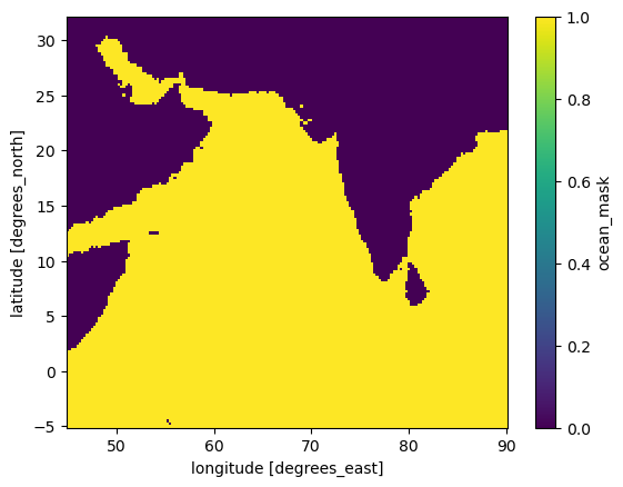
log CHL#
data_xr["y"] = np.log(data_xr["y"])
# Let's check
data_xr.sst.sel(time="2020-09-02").plot();
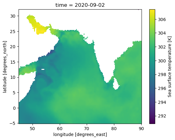
# Hmm some high chl in inland lakes
data_xr.y.sel(time="2020-09-02").plot();
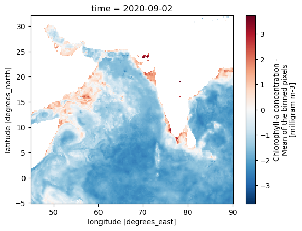
Deal with NaNs#
TensorFlow does not allow NaNs in our predictors so we need to figure out how many there are and then decide what to do about them. It looks like our predictors are fine; SST has zero NaNs or and salinity has a maximum of 79 NaN pixels on any given day. We’ll leave those days. But our response variable has some days with a lot of NaNs. We should get rid of those days with high NaNs.
# Check how many NaNs that we have

# Broadcast to 3D: (time, lat, lon) since it is 2D now
mask_3d = data_xr["ocean_mask"].broadcast_like(data_xr["sst"])

# Count NaNs over ocean only
for var in ["sst", "so", "y"]:
    var_data = data_xr[var]
    ocean_nan = np.isnan(var_data) & mask_3d
    max_nan = ocean_nan.sum(dim=["lat", "lon"]).max().compute()
    print(f"{var}: max ocean NaNs per time step = {int(max_nan)}")
sst: max ocean NaNs per time step = 0
so: max ocean NaNs per time step = 79
y: max ocean NaNs per time step = 1602
Get rid of days where our response has too many NaNs#
A rule of thumb is not to have more than 5-10% of NaNs in your response variable, otherwise the CNNs will be training on too much missingness. For us, 5% is about 800 missing pixels.
nan_thresh = 0.05 * data_xr["ocean_mask"].sum().values
nan_thresh
832.0500000000001
# Count missing CHL values over ocean for each time step in CHL
chl_nan = np.isnan(data_xr["y"]) & mask_3d
chl_nan_count = chl_nan.sum(dim=["lat", "lon"])

# Set threshold: exclude days with too much missing CHL
valid_times = chl_nan_count < nan_thresh

# Apply time filtering
data_xr = data_xr.sel(time=valid_times)
print(f"Remaining days after CHL filtering: {data_xr.sizes['time']}")
Remaining days after CHL filtering: 321
Replace data over land with NaN#
Make sure any variables over land are NaN so no lake data.
Save as a Zarr file#
Chunked & lazy loading: Keeps your Dask chunking intact.
Efficient: Only loads the data you need into memory.
Parallel IO: Works great with Dask for scalable access.
Flexible: Plays well with training pipelines in TensorFlow or PyTorch via prefetching or conversion.
data_xr = data_xr.chunk({'time': 100, 'lat': 50, 'lon': 60})
# clear encoding
for var in data_xr.data_vars:
    data_xr[var].encoding.pop("chunks", None)
<xarray.backends.zarr.ZarrStore at 0x7f6d281517c0>
type(data_xr)
xarray.core.dataset.Dataset
data_xr.to_zarr("part1.zarr", mode="w")
# data_xr.to_zarr("~/shared-readwrite/cnn/part1.zarr", mode="w")
# test
test = xr.open_zarr("part1.zarr")
test
<xarray.Dataset> Size: 104MB
Dimensions:     (lat: 149, lon: 181, time: 321)
Coordinates:
  * lat         (lat) float32 596B 32.0 31.75 31.5 31.25 ... -4.5 -4.75 -5.0
  * lon         (lon) float32 724B 45.0 45.25 45.5 45.75 ... 89.5 89.75 90.0
  * time        (time) datetime64[ns] 3kB 2020-01-01 2020-01-02 ... 2020-12-31
Data variables:
    ocean_mask  (lat, lon) bool 27kB dask.array<chunksize=(50, 60), meta=np.ndarray>
    so          (lat, lon, time) float32 35MB dask.array<chunksize=(50, 60, 100), meta=np.ndarray>
    sst         (lat, lon, time) float32 35MB dask.array<chunksize=(50, 60, 100), meta=np.ndarray>
    y           (lat, lon, time) float32 35MB dask.array<chunksize=(50, 60, 100), meta=np.ndarray>
Attributes: (12/92)
    Conventions:                     CF-1.8, ACDD-1.3
    DPM_reference:                   GC-UD-ACRI-PUG
    IODD_reference:                  GC-UD-ACRI-PUG
    acknowledgement:                 The Licensees will ensure that original ...
    citation:                        The Licensees will ensure that original ...
    cmems_product_id:                OCEANCOLOUR_GLO_BGC_L3_MY_009_103
    ...                              ...
    time_coverage_end:               2024-04-18T02:58:23Z
    time_coverage_resolution:        P1D
    time_coverage_start:             2024-04-16T21:12:05Z
    title:                           cmems_obs-oc_glo_bgc-plankton_my_l3-mult...
    westernmost_longitude:           -180.0
westernmost_valid_longitude: -180.0- lat: 149
- lon: 181
- time: 321
- lat(lat)float3232.0 31.75 31.5 ... -4.5 -4.75 -5.0
array([32. , 31.75, 31.5 , 31.25, 31. , 30.75, 30.5 , 30.25, 30. , 29.75, 29.5 , 29.25, 29. , 28.75, 28.5 , 28.25, 28. , 27.75, 27.5 , 27.25, 27. , 26.75, 26.5 , 26.25, 26. , 25.75, 25.5 , 25.25, 25. , 24.75, 24.5 , 24.25, 24. , 23.75, 23.5 , 23.25, 23. , 22.75, 22.5 , 22.25, 22. , 21.75, 21.5 , 21.25, 21. , 20.75, 20.5 , 20.25, 20. , 19.75, 19.5 , 19.25, 19. , 18.75, 18.5 , 18.25, 18. , 17.75, 17.5 , 17.25, 17. , 16.75, 16.5 , 16.25, 16. , 15.75, 15.5 , 15.25, 15. , 14.75, 14.5 , 14.25, 14. , 13.75, 13.5 , 13.25, 13. , 12.75, 12.5 , 12.25, 12. , 11.75, 11.5 , 11.25, 11. , 10.75, 10.5 , 10.25, 10. , 9.75, 9.5 , 9.25, 9. , 8.75, 8.5 , 8.25, 8. , 7.75, 7.5 , 7.25, 7. , 6.75, 6.5 , 6.25, 6. , 5.75, 5.5 , 5.25, 5. , 4.75, 4.5 , 4.25, 4. , 3.75, 3.5 , 3.25, 3. , 2.75, 2.5 , 2.25, 2. , 1.75, 1.5 , 1.25, 1. , 0.75, 0.5 , 0.25, 0. , -0.25, -0.5 , -0.75, -1. , -1.25, -1.5 , -1.75, -2. , -2.25, -2.5 , -2.75, -3. , -3.25, -3.5 , -3.75, -4. , -4.25, -4.5 , -4.75, -5. ], dtype=float32) - lon(lon)float3245.0 45.25 45.5 ... 89.5 89.75 90.0
array([45. , 45.25, 45.5 , 45.75, 46. , 46.25, 46.5 , 46.75, 47. , 47.25, 47.5 , 47.75, 48. , 48.25, 48.5 , 48.75, 49. , 49.25, 49.5 , 49.75, 50. , 50.25, 50.5 , 50.75, 51. , 51.25, 51.5 , 51.75, 52. , 52.25, 52.5 , 52.75, 53. , 53.25, 53.5 , 53.75, 54. , 54.25, 54.5 , 54.75, 55. , 55.25, 55.5 , 55.75, 56. , 56.25, 56.5 , 56.75, 57. , 57.25, 57.5 , 57.75, 58. , 58.25, 58.5 , 58.75, 59. , 59.25, 59.5 , 59.75, 60. , 60.25, 60.5 , 60.75, 61. , 61.25, 61.5 , 61.75, 62. , 62.25, 62.5 , 62.75, 63. , 63.25, 63.5 , 63.75, 64. , 64.25, 64.5 , 64.75, 65. , 65.25, 65.5 , 65.75, 66. , 66.25, 66.5 , 66.75, 67. , 67.25, 67.5 , 67.75, 68. , 68.25, 68.5 , 68.75, 69. , 69.25, 69.5 , 69.75, 70. , 70.25, 70.5 , 70.75, 71. , 71.25, 71.5 , 71.75, 72. , 72.25, 72.5 , 72.75, 73. , 73.25, 73.5 , 73.75, 74. , 74.25, 74.5 , 74.75, 75. , 75.25, 75.5 , 75.75, 76. , 76.25, 76.5 , 76.75, 77. , 77.25, 77.5 , 77.75, 78. , 78.25, 78.5 , 78.75, 79. , 79.25, 79.5 , 79.75, 80. , 80.25, 80.5 , 80.75, 81. , 81.25, 81.5 , 81.75, 82. , 82.25, 82.5 , 82.75, 83. , 83.25, 83.5 , 83.75, 84. , 84.25, 84.5 , 84.75, 85. , 85.25, 85.5 , 85.75, 86. , 86.25, 86.5 , 86.75, 87. , 87.25, 87.5 , 87.75, 88. , 88.25, 88.5 , 88.75, 89. , 89.25, 89.5 , 89.75, 90. ], dtype=float32) - time(time)datetime64[ns]2020-01-01 ... 2020-12-31
array(['2020-01-01T00:00:00.000000000', '2020-01-02T00:00:00.000000000',
       '2020-01-03T00:00:00.000000000', ..., '2020-12-29T00:00:00.000000000',
       '2020-12-30T00:00:00.000000000', '2020-12-31T00:00:00.000000000'],
      dtype='datetime64[ns]')
- ocean_mask(lat, lon)booldask.array<chunksize=(50, 60), meta=np.ndarray>
Array Chunk Bytes 26.34 kiB 2.93 kiB Shape (149, 181) (50, 60) Dask graph 12 chunks in 2 graph layers Data type bool numpy.ndarray - so(lat, lon, time)float32dask.array<chunksize=(50, 60, 100), meta=np.ndarray>
Array Chunk Bytes 33.02 MiB 1.14 MiB Shape (149, 181, 321) (50, 60, 100) Dask graph 48 chunks in 2 graph layers Data type float32 numpy.ndarray - sst(lat, lon, time)float32dask.array<chunksize=(50, 60, 100), meta=np.ndarray>
Array Chunk Bytes 33.02 MiB 1.14 MiB Shape (149, 181, 321) (50, 60, 100) Dask graph 48 chunks in 2 graph layers Data type float32 numpy.ndarray - y(lat, lon, time)float32dask.array<chunksize=(50, 60, 100), meta=np.ndarray>
Array Chunk Bytes 33.02 MiB 1.14 MiB Shape (149, 181, 321) (50, 60, 100) Dask graph 48 chunks in 2 graph layers Data type float32 numpy.ndarray
- latPandasIndex
PandasIndex(Index([ 32.0, 31.75, 31.5, 31.25, 31.0, 30.75, 30.5, 30.25, 30.0, 29.75, ... -2.75, -3.0, -3.25, -3.5, -3.75, -4.0, -4.25, -4.5, -4.75, -5.0], dtype='float32', name='lat', length=149)) - lonPandasIndex
PandasIndex(Index([ 45.0, 45.25, 45.5, 45.75, 46.0, 46.25, 46.5, 46.75, 47.0, 47.25, ... 87.75, 88.0, 88.25, 88.5, 88.75, 89.0, 89.25, 89.5, 89.75, 90.0], dtype='float32', name='lon', length=181)) - timePandasIndex
PandasIndex(DatetimeIndex(['2020-01-01', '2020-01-02', '2020-01-03', '2020-01-04',
               '2020-01-05', '2020-01-06', '2020-01-07', '2020-01-08',
               '2020-01-09', '2020-01-10',
               ...
               '2020-12-22', '2020-12-23', '2020-12-24', '2020-12-25',
               '2020-12-26', '2020-12-27', '2020-12-28', '2020-12-29',
               '2020-12-30', '2020-12-31'],
              dtype='datetime64[ns]', name='time', length=321, freq=None))
- Conventions :
- CF-1.8, ACDD-1.3
- DPM_reference :
- GC-UD-ACRI-PUG
- IODD_reference :
- GC-UD-ACRI-PUG
- acknowledgement :
- The Licensees will ensure that original CMEMS products - or value added products or derivative works developed from CMEMS Products including publications and pictures - shall credit CMEMS by explicitly making mention of the originator (CMEMS) in the following manner: <Generated using CMEMS Products, production centre ACRI-ST>
- citation :
- The Licensees will ensure that original CMEMS products - or value added products or derivative works developed from CMEMS Products including publications and pictures - shall credit CMEMS by explicitly making mention of the originator (CMEMS) in the following manner: <Generated using CMEMS Products, production centre ACRI-ST>
- cmems_product_id :
- OCEANCOLOUR_GLO_BGC_L3_MY_009_103
- cmems_production_unit :
- OC-ACRI-NICE-FR
- comment :
- average
- contact :
- servicedesk.cmems@acri-st.fr
- copernicusmarine_version :
- 1.3.1
- creation_date :
- 2024-04-25 UTC
- creation_time :
- 00:47:33 UTC
- creator_email :
- servicedesk.cmems@acri-st.fr
- creator_name :
- ACRI
- creator_url :
- http://marine.copernicus.eu
- date_created :
- 2024-04-25T00:47:33Z
- distribution_statement :
- See CMEMS Data License
- duration_time :
- PT107179S
- earth_radius :
- 6378.137
- easternmost_longitude :
- 180.0
- easternmost_valid_longitude :
- 180.00001525878906
- file_quality_index :
- 0
- geospatial_bounds :
- POLYGON ((90.000000 -180.000000, 90.000000 180.000000, -90.000000 180.000000, -90.000000 -180.000000, 90.000000 -180.000000))
- geospatial_bounds_crs :
- EPSG:4326
- geospatial_bounds_vertical_crs :
- EPSG:5829
- geospatial_lat_max :
- 89.97916412353516
- geospatial_lat_min :
- -89.97917175292969
- geospatial_lon_max :
- 179.9791717529297
- geospatial_lon_min :
- -179.9791717529297
- geospatial_vertical_max :
- 0
- geospatial_vertical_min :
- 0
- geospatial_vertical_positive :
- up
- grid_mapping :
- Equirectangular
- grid_resolution :
- 4.638312339782715
- history :
- Created using software developed at ACRI-ST
- id :
- 20240417_cmems_obs-oc_glo_bgc-plankton_myint_l3-multi-4km_P1D
- institution :
- ACRI
- keywords :
- EARTH SCIENCE > OCEANS > OCEAN CHEMISTRY > CHLOROPHYLL, EARTH SCIENCE > BIOLOGICAL CLASSIFICATION > PROTISTS > PLANKTON > PHYTOPLANKTON
- keywords_vocabulary :
- NASA Global Change Master Directory (GCMD) Science Keywords
- lat_step :
- 0.0416666679084301
- license :
- See CMEMS Data License
- lon_step :
- 0.0416666679084301
- naming_authority :
- CMEMS
- nb_bins :
- 37324800
- nb_equ_bins :
- 8640
- nb_grid_bins :
- 37324800
- nb_valid_bins :
- 9704694
- netcdf_version_id :
- 4.3.3.1 of Jul 8 2016 18:15:50 $
- northernmost_latitude :
- 90.0
- northernmost_valid_latitude :
- 82.70833587646484
- overall_quality :
- mode=myint
- parameter :
- Chlorophyll-a concentration,Phytoplankton Functional Types
- parameter_code :
- CHL,DIATO,DINO,HAPTO,GREEN,PROKAR,PROCHLO,MICRO,NANO,PICO
- pct_bins :
- 100.0
- pct_valid_bins :
- 26.000659079218106
- period_duration_day :
- P1D
- period_end_day :
- 20240417
- period_start_day :
- 20240417
- platform :
- Aqua,Suomi-NPP,Sentinel-3a,JPSS-1 (NOAA-20),Sentinel-3b
- processing_level :
- L3
- product_level :
- 3
- product_name :
- 20240417_cmems_obs-oc_glo_bgc-plankton_myint_l3-multi-4km_P1D
- product_type :
- day
- project :
- CMEMS
- publication :
- Gohin, F., Druon, J. N., Lampert, L. (2002). A five channel chlorophyll concentration algorithm applied to SeaWiFS data processed by SeaDAS in coastal waters. International journal of remote sensing, 23(8), 1639-1661 + Hu, C., Lee, Z., Franz, B. (2012). Chlorophyll a algorithms for oligotrophic oceans: A novel approach based on three-band reflectance difference. Journal of Geophysical Research, 117(C1). doi: 10.1029/2011jc007395 + Xi H, Losa S N, Mangin A, Garnesson P, Bretagnon M, Demaria J, Soppa M A, Hembise Fanton d Andon O, Bracher A (2021) Global chlorophyll a concentrations of phytoplankton functional types with detailed uncertainty assessment using multi-sensor ocean color and sea surface temperature satellite products, JGR, in review.
- publisher_email :
- servicedesk.cmems@mercator-ocean.eu
- publisher_name :
- CMEMS
- publisher_url :
- http://marine.copernicus.eu
- references :
- http://www.globcolour.info GlobColour has been originally funded by ESA with data from ESA, NASA, NOAA and GeoEye. This version has received funding from the European Community s Seventh Framework Programme ([FP7/2007-2013]) under grant agreement n. 282723 [OSS2015 project].
- registration :
- 5
- sensor :
- Moderate Resolution Imaging Spectroradiometer,Visible Infrared Imaging Radiometer Suite,Ocean and Land Colour Instrument
- sensor_name :
- MODISA,VIIRSN,OLCIa,VIIRSJ1,OLCIb
- sensor_name_list :
- MOD,VIR,OLA,VJ1,OLB
- site_name :
- GLO
- software_name :
- globcolour_l3_reproject
- software_version :
- 2022.2
- source :
- surface observation
- southernmost_latitude :
- -90.0
- southernmost_valid_latitude :
- -66.33333587646484
- standard_name_vocabulary :
- NetCDF Climate and Forecast (CF) Metadata Convention
- start_date :
- 2024-04-16 UTC
- start_time :
- 21:12:05 UTC
- stop_date :
- 2024-04-18 UTC
- stop_time :
- 02:58:23 UTC
- summary :
- CMEMS product: cmems_obs-oc_glo_bgc-plankton_my_l3-multi-4km_P1D, generated by ACRI-ST
- time_coverage_duration :
- PT107179S
- time_coverage_end :
- 2024-04-18T02:58:23Z
- time_coverage_resolution :
- P1D
- time_coverage_start :
- 2024-04-16T21:12:05Z
- title :
- cmems_obs-oc_glo_bgc-plankton_my_l3-multi-4km_P1D
- westernmost_longitude :
- -180.0
- westernmost_valid_longitude :
- -180.0
# test plot
test.so.sel(time='2020-09-02').plot()
<matplotlib.collections.QuadMesh at 0x7f6d2a41da60>
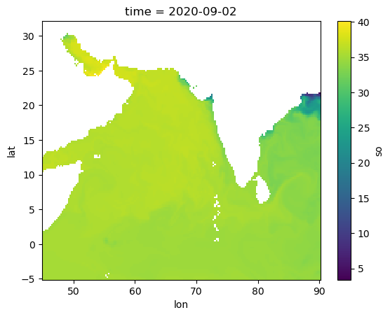
Summary#
Now we are ready to fit our CNN model.